Energy calculation in energyPRO with the MILP solver
Introduction
Flexible energy plants providing electricity, heating and cooling represent an important part of future smart energy systems based on renewable energy. Equipped with large combined heat and power units, heat pumps, electric and absorption chillers and energy storages, like thermal storages, chilled water storages and batteries, these have the possibility to provide flexibility – but an optimized dispatch of the production units is required.
energyPRO offers two dispatch methods – an advanced analytic method and a Mixed Integer Linear Programming (MILP) method.
In literature it is made probable that no single dispatch method will be able to solve all dispatch problems, therefore, an option is to make use of and combine the best of e.g. analytic and solver-based dispatch methods. This combination will even improve the dialogue with operators of DE plants, who have extensive experience in the complexity, non-linearities and constraints of the daily operation of the energy plants. We have detailed this challenge in the reviewed paper, Analytic versus solver-based calculated daily operations of district energy plants (1).
In this How To Guide the MILP method is described. We have in the guide shown complicated examples where the MILP performs well, e.g.:
- Trigeneration plant with both hot water and chilled water storages
- Carbon Capture and Utilization plants
- Hybrid windfarm, PV and battery plants with restricted access to the electrical grid
What is a MILP Solver
Mixed Integer Linear Programming Solver finds solutions to problems specified as:
Where:
- \(x\) – vector of variables
- \(c^{T}\) – vector of coefficients of the objective function
- \(A\) – matrix of variables’ coefficients in the inequality constraints
- \(b\) – vector of constants used in the inequality constraints
- \(A e q\) – matrix of variables’ coefficients in the equality constraints
- \(b e q\) – vector of constants used in the equality constraints
- \(l b\) – vector of lower bounds of variables
- \(u b\) – vector of upper bounds of variables
- \(x_{i}\) – integer variables
In other words, MILP Solver finds the solution to a problem defined with linear constraints and objective function, where some of the variables can be binary or integer. The ability to describe an energy system with a set of linear constraints enables the use of a MILP Solver as a calculation method in energyPRO.
Advantages of the MILP Solver method
The main advantage of a MILP Solver method is the accuracy of solution. If the problem is defined well the solution found with use of MILP Solver is the optimal solution of the problem.
The other advantage is that the optimal dispatch is found without the need to adjust the operating strategy of the units.
The default solver – HiHGS
The HiGHS (recommendedf) and CBC are included with energyPRO. The commercial solvers Gurobi and CPLEX can be used if available.
Setting up a calculation with MILP Solver
The user can decide on the method used for the calculation – Analytic or MILP Solver. This chapter presents how to set up a calculation with MILP Solver.
Choosing MILP Solver as method for calculation
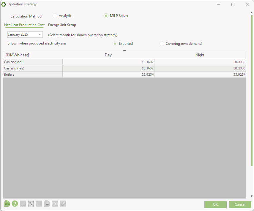
The calculation method can be chosen in Project identification or Operation strategy window.
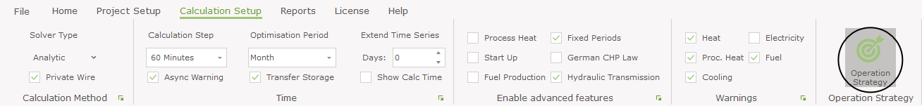
The easiest approach is to select the "Calculation Setup" tab, then choose "Operational strategy" from the ribbon menu. To perform the calculation with MILP solver, "MILP Solver" must be chosen in "Calculation Method" field.
Setting parameters of MILP Solver
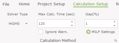
It is possible to change two parameters of the calculation with use of the MILP Solver in energyPRO. This can be done in the "Calculation Method" section in "Operational strategy" window.
Max. Calc. Time (sec) – indicates the maximum time of one calculation. One calculation is considered to cover the length of optimization period. If the length is chosen to be Month and the project is calculated for a year, 12 calculations are going to be performed. The Max. solution time will not affect quick calculations but will stop the optimization if it did not reach a solution with wanted precision within the specified time. The default value is 120 seconds.
Gap (%) – indicates the precision of calculation which must be reached to stop it. The gap may be interpreted as an indicator of how far the solution is from the optimal one. It is a very important parameter and may highly influence the time it takes to obtain the result. If the gap is set to be a very small number, the calculation may take a long time. It is because the calculation will not be stopped until the Wanted precision is reached or the Max. Calculation time exceeded. The default value of Gap is 1%.
Usually, a feasible solution of the problem is obtained in the first iterations of simulation. Most of the times this solution is far from the optimal, but it satisfies all constraints of the system. The MILP Solver attempts to improve the feasible solution in the next iterations.
Warning and possible solution
If the Max. calculation time is reached and the gap is not met, a warning is displayed. It indicates all the calculations for which the time limit was reached and the Precision of the calculation. The solution displayed in energyPRO, after the warning, is the best feasible solution achieved within the time limit. To reach the wanted precision the user should consider increasing the Max. solution time. To speed up the calculation it is advised to decrease the wanted precision (enter a larger percentage).
The warning may be disabled in MILP Settings by selecting the checkbox Ignore warn.
Using other solvers than the default HiGHS
The default MILP Solver, included in energyPRO installation, is HiGHS. It is an open-source MILP solver, which proved to have the best performance out of the available open-source MILP Solvers. Nevertheless, in highly complicated simulations the commercial MILP Solvers prove to be more efficient. Therefore, a possibility to use two of the commercially available Solvers is included in energyPRO, Gurobi and CPLEX.
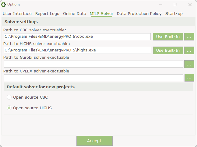
The solver can be changed in Options in energyPRO setup menu as presented below. The change is not project specific but is introduced in all the projects.

In Options the MILP Solver tab should be selected. To change the MILP Solver Gurobi must be chosen as presented below. The field Path to solver executable should include the path to gurobi_cl.exe file on the user’s computer. If the installation of Gurobi was done with default settings the path should be similar to the one below. However, it may vary between versions.
Limitations of the MILP solver
This chapter presents the functions, which are not implemented in the calculation with MILP Solver or are implemented with limitations.
1.Modelling of “Production to store not allowed”
The current implementation of the constraint has a limitation. If the unit is not allowed to produce to store but is allowed to transmit to other sites, the solution generated by solver will not prevent that the transmitted energy to the other sites is stored in these sites.
3.Non-linear objective functions
A payment expressed with non-linear equation cannot be used when MILP Solver is used as a calculation method. Non-linear terms are all the terms where two or more variables are multiplied. Obviously, the variables can be multiplied by constants such as coefficients or prices.
4.Limited implementation of max(), min() and if() functions
The implementation of the \(max()\), \(min()\) and \(if()\) functions is very limited when MILP Solver is chosen as the calculation method. In the current approach it is done by stepwise assuming that 1 MWh of a certain energy type is produced or consumed by a certain production unit, when all others are zero. An example with \(max()\) function implementation is:
The payment:
This payment will thus to the electricity produced by \(BiogasCHP\) in a certain time step add to the objective function:
This payment will thus to the electricity consumed by \(HP\) in a certain time step add to the objective function:
This implementation can create inaccurate objective functions. Therefore, it is advised to avoid using these functions in the payments when MILP Solver is chosen as the calculation method.