Energy calculation in energyPRO with the analytic solver
This chapter describes how energyPRO calculates an optimal operation of an energy plant with the analytical method. For a short overview also see this tutorial video on our homepage.
The optimisation problem
energyPRO is a powerful tool in which you can model complicated energy systems, consisting of an unlimited number of demands and energy conversion units.
The model of the energy system and the applied operation strategy (user defined or auto calculated) determines the productions and consumptions of the production units. energyPRO helps making the productions optimal, for instance by easy accessible ways of changing the modelled energy system and operation strategy. Sensitivity analyses is easily done by the use of energyPRO.
It is important to keep in mind that optimising a local energy plant is often a complex task.
Normally, the demand for electricity is high in the morning and in the afternoon, lower during the rest of the day and lowest during night time, weekends and holidays. Reflecting on this, the prices paid for the produced or consumed electricity may vary significantly with the time of the day. On the other hand, a heat demand is normally low during summers and many times higher during winters, and a cooling demand will normally be higher in the summer periods and lower in the winter periods.
A thermal store or cooling storage is one way of solving this mismatch between the need of electricity and heat/cooling. Another way to add flexibility is to add heat blow-off capacity allowing electricity producing energy units to be used more flexible.
Another complexity is that fuel, e.g. biogas, can be restricted in amount and eventually stored in a fuel-storage. A CHP unit might for instance be able to use two types of fuel e.g. biogas and natural gas, where the biogas is restricted in amount and can be stored in a biogas-storage and the heat can be stored in a thermal store. An energy unit might be operated with or without an economizer.
Another complexity can be that the electricity production is restricted to a certain demand for electricity e.g. the electricity demand in a town. Furthermore, electricity consuming heat pumps increase the complexity of energy system calculations.
energyPRO makes it possible to analyse optimal solutions, considering all the above-mentioned factors.
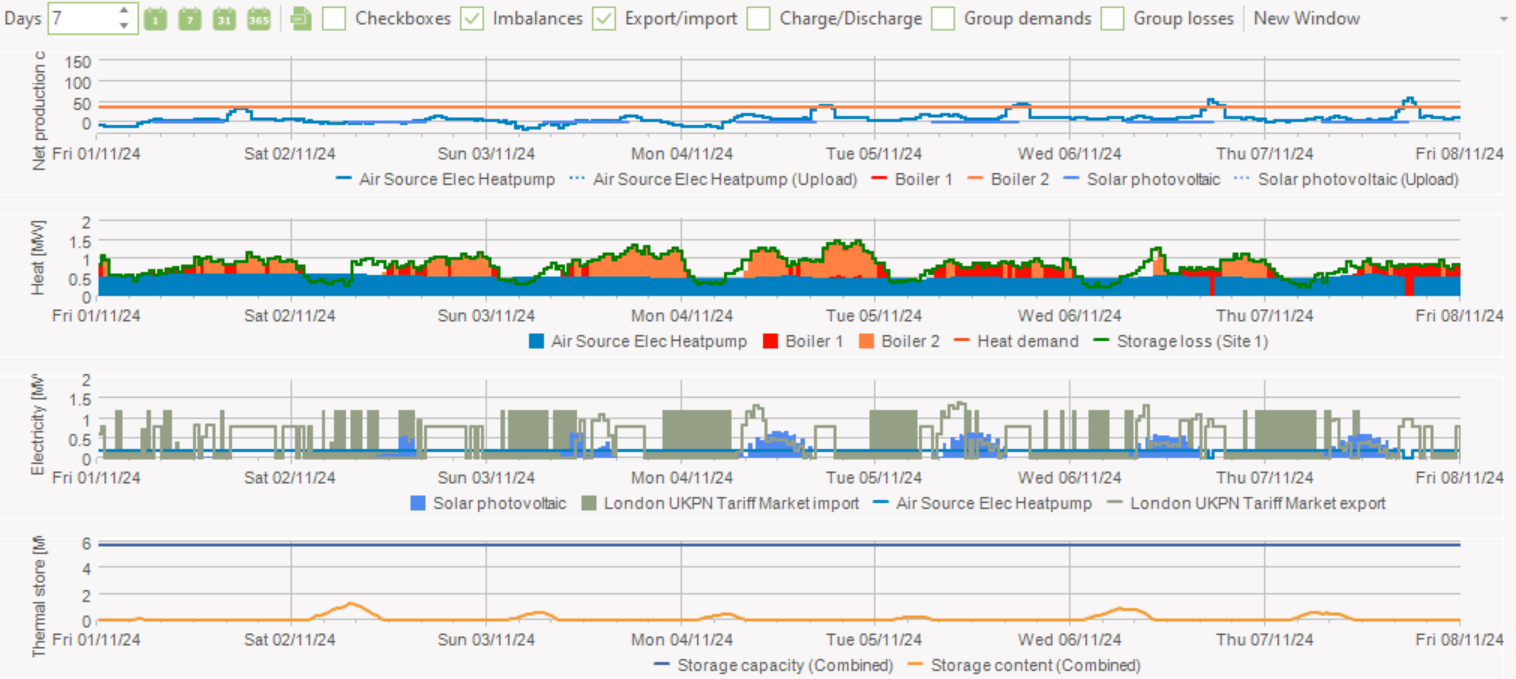
In the shown example it is assumed, that the demand for electricity is highest in the daytime (high tariff). During night time, in the weekends and on official holidays the demand is reduced even further (low tariff) - The price structure for the electricity production reflects this variation, and hence the priority numbers (Net Production Costs) in the top graph are lower for the units in the day time compared with the night time and weekend.
The heating demand is low during the summer and much higher during the winter. A thermal store is used to solve the temporal displacement between the demands for electricity and the demand for heating.
Time series is a fundamental object in energyPRO
Project information has to be available and the energy system has to be modelled, before energyPRO starts calculating optimal energy productions. Directly and indirectly time series are playing a core object in all energyPRO models. This could be weather data, demands, electricity prices, results etc.
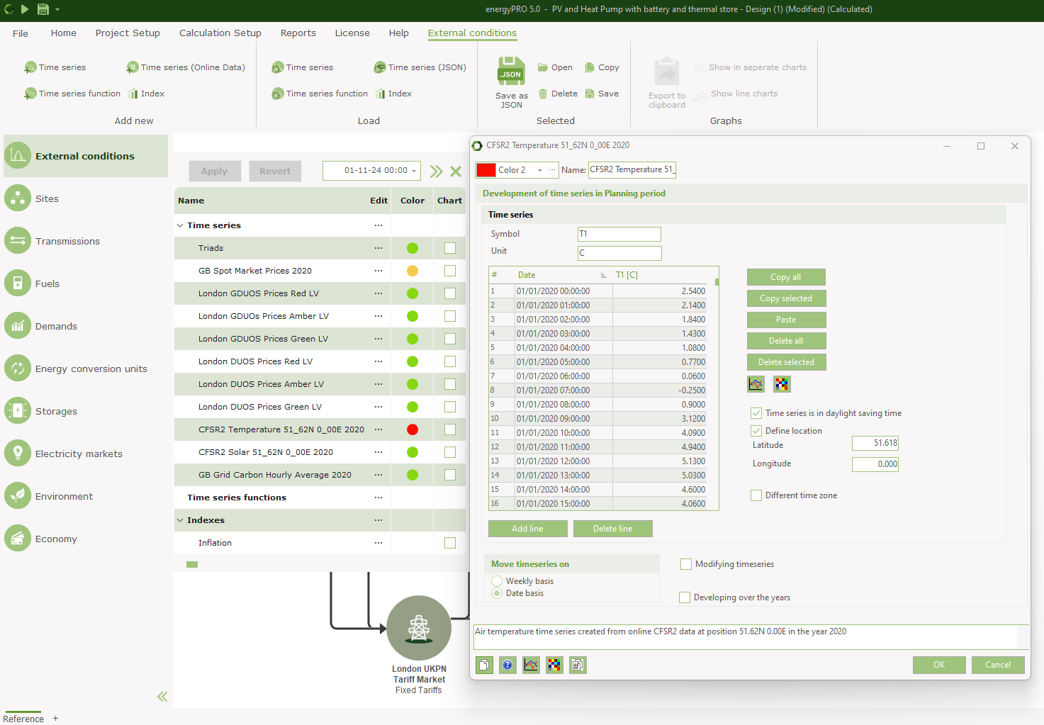
A time series consists of a symbol, a unit and a set of points consisting of Date, Time, and Values
When you have made a new time series, this time series is available both to model the variation of demands, to influence the power curves of production units and to describe electricity prices on the spot market.
During an energyPRO calculation the calculation period is split in to fixed calculation steps where everything is constant. The size of this step is controlled in the Project Identification. If your time series do not match the specified calculation step, energyPRO will calculate mean values or closest values for a given calculation step.
energyPRO automatically extends your time series
If you have described in an energyPRO-model, that demands or production units depends on some external condition (e.g. ambient temperature), energyPRO needs to know for the complete planning period, the values of this external condition. The hard way of doing this is to create your own time series for the complete period. This will normally be inconvenient and unnecessary.
Often you have access to information for a period of one year, which you want to extend to the whole planning period - this will automatically be done within the energyPRO calculation.
The extension is based on the following principles.
Within one specific year: A time series is well defined between the first time (start time) and the last time (end time). Outside start time and end time, the value is identical with the value at the end time.
From one year to another year. There are two options for extension of time series.
- The extension is weekly based.
- The extentison is date based
Option a). This means that Monday in week 2 will adopt the values from Monday in week 2 in the nearest year, etc.
energyPRO follows the ISO week date system, where each week begins on a Monday.
There are special conditions around New Year. If a given weekday in week 1 in the planning period is not present in the time series, the value for the weekday in week 2 is used. If a given weekday in week 52 in the planning period is not present in the time series, the value for the weekday in week 1 is used. If Monday to Tuesday in week 53 in the planning period is not present in the time series, the value for the weekday in week 52 is used. Finally, if Friday to Sunday in week 53 in the planning period is not present in the time series, the value for the weekday in week 1 is used.
The main reason for making the time series weekly based is that some variation described in time series often varies systematically within a week. E.g., electricity demands in weekdays are often significantly different from electricity demands in weekends.
Option b). This means that e.g. February 2nd 2014 is equal to February 2nd 2015.
Demands are also time series
In energyPRO, it is not obvious, that demands are time series, identical to time series for external conditions. That is because you get a lot of help to model the variation of a demand.
But if you convert this demand to time series it becomes obvious, that a time series for a demand is exactly identical to time series for external conditions, also being available by formula expressions to influence the power of production units.
Modelling variation of demands with use of a fixed profile of demand
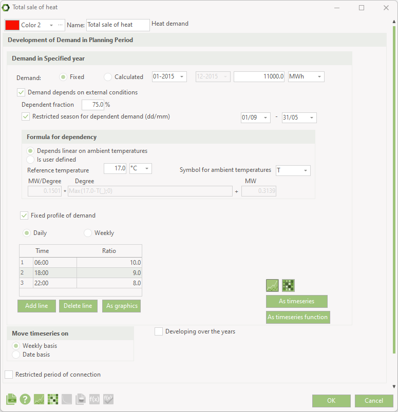
It is possible to state that a demand has to follow a fixed profile of demand. See the bottom table in the editing window on Figure 33.
If a fixed profile of demand is chosen, daily or weekly, then the demand time series created so far will be modified. The main principle is that the demand on daily (or weekly) basis will remain unchanged, but the distribution within the 24 hours a day (or week) will be redistributed so it follows the stated fixed profile of demand.
Priorities are calculated in each time step
Before the energy calculations each productions unit get a priority in each time step. This is done automatically based on the payment lines or is done user defined.
Depending on the electricity wholesale market type (fixed market or spot market) this is done different. When using a fixed tariff timesteps are grouped into subgroups defining different tariffs elements. When calculation spot market calculation this division into subgroups are not needed.
Fixed Tariff. Group time periods for optimization
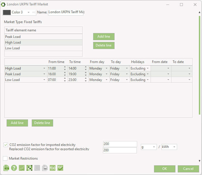
In “Electricity markets”, the time periods can be divided into groups. Such a division is often convenient if electricity prices vary systematically. Each group is labelled by a “Priority name”. In the figure below, there are three priority names. “Peak Load”, “High Load” and “Low Load”. The grouping of the periods is specified by mean of the lower table. The example will divide a year into hundreds of time periods during a year.
This information is used when the operation strategy is designed.
Spot market
When preparing a spot market calculation there is no subdivision into groups. The core element is a time series holding the spot prices. In the automatic calculation strategy the price is each time step is used when calculating the priority for a specific energy conversion unit in a specific time step.
Energy conversion units
There are two sorts of energy conversion units. The options are a production unit and a heat blow-off unit
Production unit
Regarding the energy conversion calculations the production units contain the definition of the power curves and eventually some time restrictions.
A production unit is described by a set of power curves, which varies for different types of production units. The optional curves are:
- Fuel consumption
- Fuel production
- Heat production
- Process heat production
- Heat consumption
- Process heat consumption
- Electricity production
- Electricity consumption
- Cooling production
- Fuel production
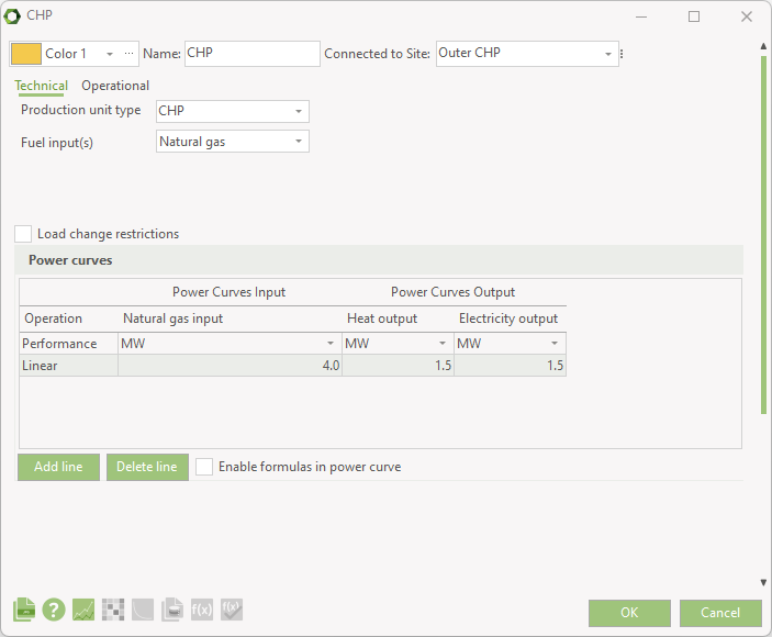
A standard CHP unit with three power curves: Fuel (consumption), Heat (production) and Electricity (production)
The power curves are described by one or more lines which together define a set of continuous curves. All numbers in a specific line has to be less or equal to the equivalent value in the line above. The upper line states maximum load, while the lower curve states the minimum load.
The power curves might vary from one time period to the next (the power curves might be a function of external conditions, for instance the return temperature of district heating water or the ambient temperature.
If the power curves are described by only one line it implies that there automatically has been assumed added an extra line containing only zeroes, describing the minimum load (if part load is allowed in the operation strategy).
It is also possible to state that the production on a specified production unit depends on other units which can be done either by checking “Operations dependent on other unit” or checking “Enable formulas in power curves” and then using the PaP-functions in the power curves.
Heat rejection unit
A heat rejection unit is described by a constant heat rejection capacity all year.
In the Operation strategy you must state, which production units have access to the heat rejection unit.
Thermal storage and cold storage
A thermal storage and cold storage is in each time period defined by a maximum content measured in MWh of either heating or cooling. In the Operation strategy, you have to state, which production units have access to these storages.
The Operation strategy (example with Fixed tariffs – User defined)
The operation strategy consists of two main tabs (three or four if the model contains both a heating demand and a cooling demand and/or fuel producing units). These are “Heat (or cooling, or Fuel) Production Strategy” (or “Net Heat/Cooling Production Cost” when automatic operation strategy are chosen) and “Energy Unit Setup”.
Priorities of production section
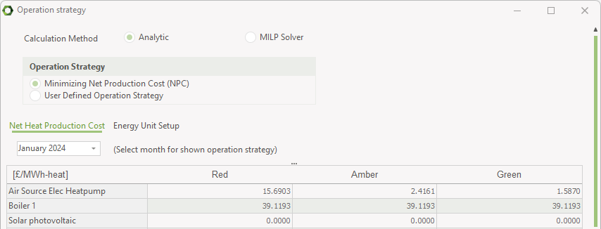
In the “Priority of productions” table in the “Production Strategy” tab you find a matrix consisting of Priority periods specified in the “Electricity markets” editing window in the column dimension and the defined production units in the row dimension.
Above it is seen that the production from the Air Source Elec Heatpump is prioritised across all the three periods, indicated by the lowest numbers. In the example, the boilers are always prioritised after the Air Source Elec Heatpump, and are only allowed to produce if the Heatpump is not able to produce all the heat needed in the three periods.
Given the matrix above, energyPRO now first calculates Heatpump in the sppropriate period and then the two boilers.
Note that if no number is attached to an element in Priority of Productions table the production unit will not operate in that specific priority period, this is shown for the solar photovoltaic.
Heat rejection allowed
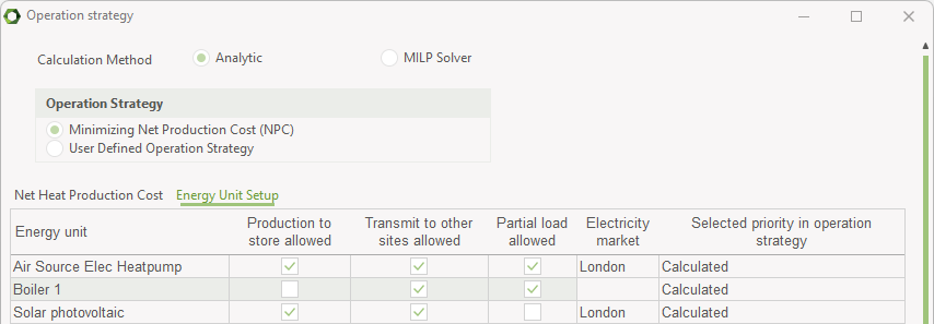
In the “Heat rejection allowed” table in the “Energy Unit Setup” tab you can define which energy conversion units are allowed to reject heat, if the heat cannot be utilized or stored. This table is only shown if a “Heat rejection” has been added.
Miscellaneous
In this section of the “Energy Unit Setup” tab is specified another matrix, horizontally consisting of some options and vertically of the defined production units. The options are:
- Production to store allowed (only if a thermal or cold store is defined)
- Production transmitted to other sites (only if there are more sites in the project)
- Partial load allowed
- Selection of electricity market
Calculating a time period under restrictions
A usual method of calculating energy productions would be making a chronological hour for hour calculation, taking into account, that e.g. producing in the night might fill the thermal store too early, prohibiting more attractive productions to be placed the day after in the morning.
To secure productions in the most favourable periods, energyPRO does it the opposite way. It starts producing in the most favourable periods, not doing it chronologically. This has the consequence that each new production has to be carefully checked to make sure it does not disturb already planned productions, before being accepted.
The year is divided into a fixed number of time periods (depending on the calculation step), which are all tested for possible productions.
In this section it is described, how optimal production from a production unit is planned in one time period and it is described how a sufficient derating (reduced load) is determined.
As a starting point, an attempt is made to keep the production unit running by sufficient derating the load of the production unit in the whole time period in order to reduce the number of starts.
The ability to derate the load might be limited for two reasons. The first reason being that if partial load is not allowed (miscellaneous section in Operation strategy). The second reason is the possibility that a minimum load appears on the power curve(s).
Taking into account dependency on another production unit
It is possible to state, that production of a unit is only allowed, if no production is planned on another production unit. If there in a certain time period is already planned production on the specified unit, no production will be possible on the second unit.
Contrary to this, it is possible to state, that production is only allowed, if production on a second unit is already planned. If there in a certain time period is planned production on a second specified production unit, the considered unit is allowed to operate, otherwise not.
Production may be limited to electricity demand
In the Operation strategy it is possible to state that the project should run in Island Operation mode with no exchange to the electricity market. In this case electricity production must be limited to the electricity demands. The allowed electricity production is calculated by taking the electricity demand then adding the electricity consumption from higher prioritised production units and finally subtracting the electricity production from higher prioritised production units. The considered production unit is derated, so that it does not exceed the allowed electricity production.
Limitation in heat and cooling production
It is controlled, that the derating of a production unit is sufficient, so that already planned future productions are not disturbed. That is to say that the thermal or cooling storages are not overfilled in the future due to the heat or cooling production in the considered time period.
If production to thermal or cooling storage is not allowed for a specified unit in the Operation strategy, the heat or cooling production from that production unit must not change the planned use of the thermal or cooling store.
If you have chosen in the Operation strategy, that the production unit has no access to a heat rejection unit (cooling tower), the heat production from the production unit must not change the planned use of the heat rejection unit in the future.
Limitation in fuel consumption
It is controlled, that the derating of a production unit is sufficient, so that already planned future productions are not disturbed. That is to say that there is sufficient fuel in the fuel storage in the future for already planned productions.
If it is possible to reduce load, so that the above-mentioned limitations are met, a new planned production has been found and accepted.
Planning of new productions follow Operation strategy
The Operation strategy is where you choose the superior priority of productions. Priority numbers states the order of productions. The units are calculated by increasing numbers. I.e. the unit with the lowest number is calculated first. All possible production on a unit is fully obtained before production with the next unit (with the next priority number) is examined and calculated.
Reducing number of starts
Given the above priority information there will be a lot of time periods with the same priority and these could simply be started chronologically which would give a ”correct” result with regards to energy conversion. However, we have experienced that the chronological approach produces too many starts which is not desirable since most production units will have some kind of start cost.
Reducing starts by giving priority to expansion before new starts
If at a given time during an optimization there is both the possibility to expand an already started block and start a new block with the same priority we will always select the expansion before starting a new block. This is of course only the case if the expansion can be done under all the restrictions mentioned in Methods, Analytical Method, Restrictions.
Reducing starts by adding start costs
In the payment lines for a production unit it is possible to add a start cost for each time the unit is started. If such a start cost is defined it will influence the priority of that unit during the optimization. The start cost is simply added to the priority of that unit and thereby making it even more undesirable to start that unit compared to expanding the unit in already started blocks.
As an example please consider the scenario during an optimization where we can either expand a block at priority 56 or start a new block at priority 45 (without start cost added). Without start costs it is cheapest to start the new block. If we then have a start cost of 20, the new priority for starting up would be 45+20 and hence we now prefer to expand at priority 56 instead.
Reducing starts by merging already started blocks
Now that start costs can prevent us from starting new blocks we can also consider the other scenario where we want to merge two blocks in order to remove one of the starts. During the optimization we will continuously look at whether two blocks can be merged to remove a start. The time periods in between the blocks might not have a good enough priority from the operation strategy to be started, but given the fact that we will remove a start we now increase their priorities according to the removed start cost.
Reducing starts by looking for empty heat or cold storage
Even with the start cost considerations there will still be situations where we see too many starts because a production unit keeps starting up every time it “sees” that there is room for it in the heat or cold storage. To prevent these starts we will always delay a start until the heat or cold storage is empty as long as the priority is the same in the next calculation step. This ensures that when the unit is started it can keep running for as long as possible (it could still be restricted by other things).
Reducing starts by looking for full fuel storage
In the same way a unit could keep starting for a short while whenever there is enough for it to run in the fuel storage. So in this case we will delay the start until the fuel storage is full (again given the next calculation step has the same priority). This gives the unit the longest start block without being restricted by the fuel input.