Method of hydraulic transmission calculation in energyPRO
Restrictions in the hydraulic calculation
The transmission temperatures are decided as external conditions, i.e., no tempera-ture optimization is included.
Input for the hydraulic calculation
General constants
- Specific heat capacity of water, \(C_p\)
- Density of water, \(\rho\)
- Time step in optimization period, \(\bigtriangleup T\)
- Gravitational acceleration, \(g\), [\(9.82 m/s^2\)]
Input for each site
Two inputs are present in the calculation method:
• Supply temperature, \(T_{sup}\)
• Return temperature, \(T_{ret}\)
\(T_{sup}\) is understood as the minimum temperature needed in the site. It can be de-termined by the minimum temperature needed to supply heat demands, minimum temperature at which a unit at the site produces heat or minimum temperature at which a unit at the site consumes heat.
\(T_{ret}\) is understood as the mixed temperature returning from heat demands in the site or from transmission lines to the site.
Input for each transmission
Five inputs are present in the calculation method:
- Length of transmission, \(L\)
- Internal diameter of forward and return pipes, \(d\)
- Specific heat loss, \(U\)
- Pipe roughness, \(\epsilon\)
- Ground temperature, \(T_g\)
Temperature zoning in a hydraulic calculation in energyPRO
The sites and transmissions are divided into temperature zones. Each site and each transmission belong to only one of the temperature zones.
If the energy can flow from one site to another site through certain transmissions and can flow back through certain transmissions, all the sites connected by the transmissions, and the transmissions in which the flow may happen, are in the same temperature zone. Such a system can be formulated as a graph with strongly connected components.
One-way transmissions are always in the same zone as the site from which the transmission is possible. If there is a site to which no energy flow back is possible, it is together with the outgoing transmission, in their own temperature zone.
In each temperature zone the sites and transmissions are operated at the same supply temperature, \(T_{sup}\), and return temperature, \(T_{ret}\). This is done by choosing the highest supply and highest return temperature from all the sites in the temperature zone. These operation temperatures in each temperature zone can change from time step to time step.
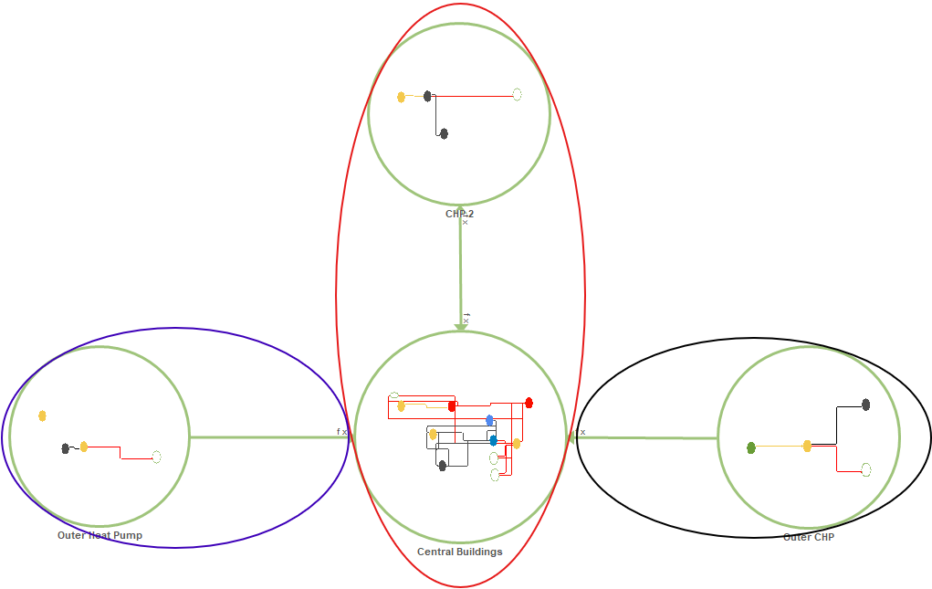
Example presented above has three temperature zones. \(T_zA\) (Blue) and \(T_zC\) (Black) are created because there is no energy flow back to Outer Heat Pump or Outer CHP and the outgoing transmissions form a temperature zone with the source sites. \(T_zB\) (Red) connects two sites, where the energy can flow out of and back again to every of the sites.
The supply and return temperatures in the presented example, entered in the sites, are shown in the table below. For simplicity these are assumed to be constants but entering them as timeseries is also possible.
| Site nr | \(T_{sup}\) [°C] | \(T_{ret}\) [°C] | |
|---|---|---|---|
| 0 | Central Buildings | 70 | 35 |
| 1 | Outer Heat Pump | 60 | 35 |
| 2 | Outer CHP | 60 | 40 |
| 3 | CHP 2 | 90 | 50 |
As previously described, \(T_{sup}\) and \(T_{ret}\) in a temperature zone are chosen as maximum values entered in the sites belonging to the considered temperature zone. In the considered example we have one temperature zone with more than one site – \(T_zB\). \(T_{sup}\) and \(T_{ret}\) for all sites in \(T_zB\) are summarized in the table below and in the last column the maximum values are highlighted.
| Temperature zone B | ||||
|---|---|---|---|---|
| New town | Solar Site | Old town | Operation temperatures in temperature zone | |
| \(T_{sup}\) [°C] | 60 | 60 | 60 | 100 |
| \(T_{ret}\) [°C] | 35 | 40 | 40 | 40 |
The operation temperatures in the temperature zone in the table above is possible to be realised sufficiently precise in a real system.
If e.g., the energy flows from Old town to New town, you can shunt the 100°C arriving at New town with colder water to get the 70°C, and you can shunt the 35°C returning from a demand in New town with warmer water, to bring it to the 55 °C of the return temperature in the temperature zone.
In \(T_zA\) and \(T_zC\) there is only one site. This means that the supply and return temperatures in \(T_zA\) are the same as the one specified for HP Site. The same goes for \(T_zC\), where the supply and return temperatures are equal to the ones specified in CHP Site.
A warning is given if an energy flow is indicated possible from a temperature zone with lower \(T_{sup}\) to a temperature zone with higher \(T_{sup}\). Therefore, in the presented example we would have a warning because \(T_{sup}\) from \(T_zA\) and \(T_zC\) is lower than the one in \(T_zB\) and the flow form \(T_zA\) and \(T_zC\) to \(T_zB\) is possible.
Maximum allowable velocity in the pipes for transmission capacity calculation
The maximum allowable velocity in the pipes will act as an energy flow boundary condition and the transmission energy flow in a pipe will be constrained to be within this value.
The maximum allowable velocity in the pipe usually depends on the pipe nominal diameter and the typical values are given in the table below. These values are selected as industry standard as higher velocities have been known to cause noise problems and damage internal layer of pipes.
| Nominal diameter | Maximum allowable velocity, \(V_{max}\) |
|---|---|
| DN 20-400 | 2 m/s |
| > DN400 | 3 m/s |
Knowing the maximum allowable velocity, the maximum allowable energy flow rate in the pipe can be determined by
Where \(m_{max}\) is the maximum allowable flow rate, \(v_{max}\) is maximum allowable velocity obtained from the table above and \(d\) is density.
To implement the boundary condition for maximum energy flow, the transmission variable is defined as follows.
Where, \(TR_{max}[i,j,t]\) is the max transmission from site \(i\) to \(j\) in time step \(t\), \(m[i,j,t]\) is the corresponding mass flow rate from site \(i\) to \(j\) in time step \(t\), \(C_p\) is specific heat capacity of water and \(T_{sup}\) and \(T_{ret}\) is supply and return temperatures in the temperature zone.
Maximum allowable pressure gradient for capacity calculation
Pressure losses are mainly due to frictional resistance. Calculating the Reynolds number for the flow is the first step. The procedure for calculating the Reynolds number is described as
Where, \(\mu\) is the dynamic viscosity, \(V\) is the volume flow rate, \(v\) is the corresponding flow velocity and \(Re\) is the Reynolds number. For district heating systems the flow is between transitional and fully developed turbulent flow with Reynolds number being higher than 104. The Darcy friction factor for such flows can be estimated using Serghide’s method [2], which is similar to the paper by Gudmundsson 2021:
Where, \(f\) is the Darcy friction factor [-] and \(\epsilon\) is the pipe roughness [m]. Thus, the pressure loss of the system and the friction pressure gradient can be calculated as:
Where, \(\bigtriangleup P\) is the major pressure loss and the pressure gradient is obtained by dividing it by the pipe length.
The boundary condition for the maximum allowable pressure gradient in the system is a user input. The default value for most systems is 100 Pa/m and rarely goes up to 150 Pa/m in transmission pipes [6]. The calculated friction pressure gradient obtained from equation is compared with the maximum allowable value and converted to \(TR_{max}[i,j,t]\) as described in section 3.7.4.
Heat Loss calculation
A typical transmission pipe cross section representing the insulation and casing as shown below.
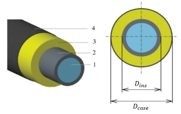
The heat loss in a pipe is calculated with the following formula.
Where \(T_{sup}\) and \(T_{ret}\) is supply and return temperatures in the temperature zone. \(T_g\) is ground temperature. \(U\) is the specific heat loss.
Calculation of total pressure drop
The total pressure drops in supply and return pipe can be calculated using a simplification: the pressure gradient in supply and return pipe are equal.
The calculation method presented in Methods, Hydraulic transmission, Maximum pressure gradient are used to calculate the pressure gradient (\(PG\)) in supply pipe, thus making the assumption that the pressure gradient is equal in supply and return. Hence, the following formula can be used for calculation of total pressure drop in a transmission line:
Work of pumps
A rough estimation of the needed work from pumps can be made by assuming that the pumps need to cover the total pressure drop. This assumption will cause an underestimation of the work, since no information about the pipes are considered (bends, valves etc.). To estimate the work of pumps the following formula can be used:
Where both \(TotPressDrop_{Trans}\) and \(V\) are different values for each time step.