External conditions

The “External conditions” folder serves as parent folder for indexes and time series and time series functions.

Time series

Time series are the fundamental data format in energyPRO. Time series relates very closely to spread sheet formats. You can copy a time series to spread sheet and you can copy a time series from a spread sheet.

A time series consists of set of values each connected to a specified date and time. The External conditions time series can be accessed from several of the other editing windows in which the project is specified.

A typical time series example is a series to distribute a heat demand by using a time series holding the ambient temperature. Other examples of using time series are the calculation of the production of a solar plant by using a time series holding the solar radiation, and a time series holding electricity spot prices used for specifying “Electricity market” prices.

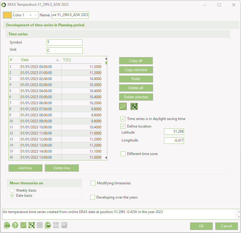
Example: Temperatures in London

Symbol

The symbol is a unique short name for the time series. The symbol is used for referencing the time series elsewhere in the energyPRO. All time series, time series functions and indexes, used in a project, must each have a unique symbol.

Note: The symbol is repeated in the header of the editing window.

Unit

The unit in which, the values in the time series, is stated. The unit is for presentation use only and is not evaluated during calculations.

Time series

Time series consist of rows all specified with the two fields; date/time and value. Arbitrary length of periods between every element in the time series is allowed.

The function of the buttons:

• Copy all: Copy all values from the actual time series to the clipboard. From the clipboard, the values can e.g. be pasted into a spread sheet like Excel.
• Copy selected: Copies selected row(s) from actual time series into clipboard. Selection is to be done by use of the keyboards arrow-tabs or by mouse.
• Paste: Pastes the content from clipboard to the time series table. Make sure you are pasting using the correct format; date/time and value. For more on importing data from a spread sheet to a time series in energyPRO, see appendices A.
• Paste Wizard: Which opens the "Time Series Import Form" with more options for pasting data.
• Delete all: Deletes all values in the time series.
• Delete selected: Deletes selected row(s) from the time series. Selection is done by using either the keyboards arrow-tabs or the mouse.
• Show graphics: The “Show in graph viewer” button gives a graphic representation of the time series table.
• As Carpet:
• Add line: Add a new line below the active line
• Delete line: Deletes the active line

Time series is in daylight saving time

If the time series is in daylight saving time, enable this checkbox. This will typically be the case for price time series, such as electricity spot prices and electricity balancing prices.

Typically time series not in daylight saving time are meteorological time series.

Define location

This checkbox has to be enabled if the time series contains solar radiation values and is used in a solar collector or photovoltaic.

The latitude and longitude are specified in decimal degrees. The latitude has positive values north of equator and negative values south of equator. The longitude has positive values east of Greenwich Mean Time (UTC) and negative values west of Greenwich Mean Time.

Different time zone

If the time series is in a different time zone than the time zone of the project, this checkbox is selected.

This gives the same options as in External conditions.

A typical case can be meteorological data measured in UTC time.

Converting time series according to time zone and daylight-saving time

If the time series is in a different time zone it is converted according to the difference in UTC offset.

If the projects time zone is with daylight saving time and the time series is with daylight saving time the time series is not changed. If the time series is in standard time the values are moved one hour forward in the daylight-saving time period.

Likewise, if the projects time zone is without daylight saving time and the time series is in daylight saving time the values are moved one hour backward in the daylight-saving time period.

When the upper “as Graphics” button is pressed a graphic view of the data is shown as specified in the table. Below is an example, where the time series containing daily temperatures in London is represented graphically.

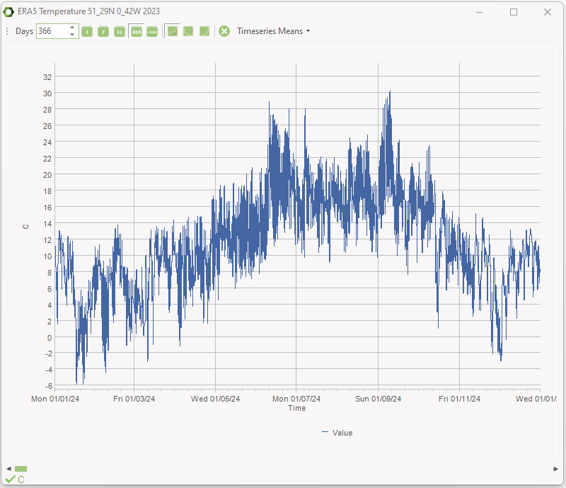
In the top of the window, you have the option of select a number of predefined days in window:

Also, you have the option of viewing the time series as duration curve.

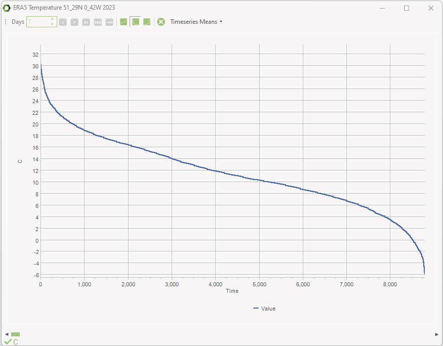
Beside the option of selecting days to show in the graph window, you can click and drag right and down to zoom in.

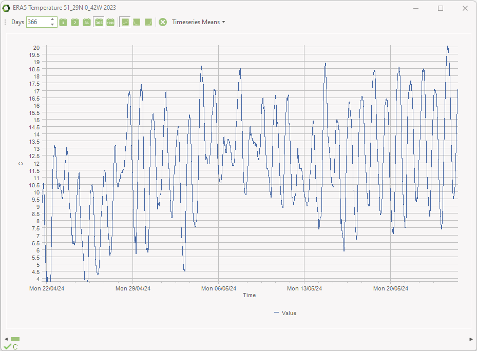
By click and dragging to the left and up, you zoom out again.

There is an alternative graphic view, Carpet. This view has the days on one axis and hours on the other axis. The Carpet view seen below show an example solar radiation for London. This view show not surprisingly that the solar radiation is concentrated in summertime and round midday.

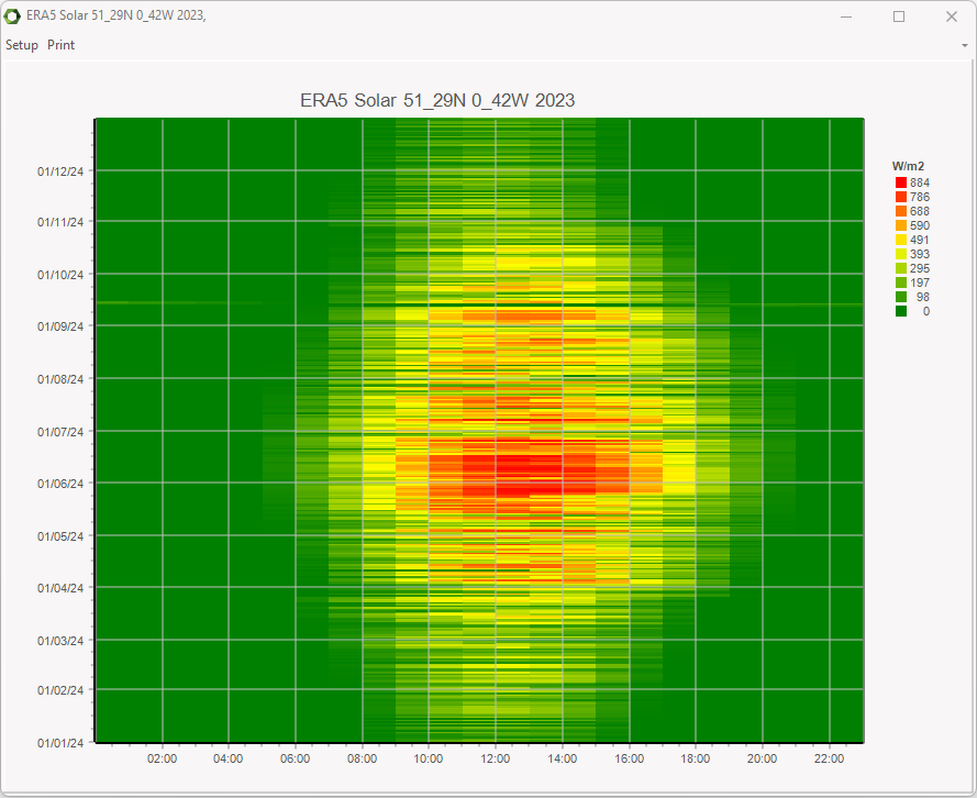
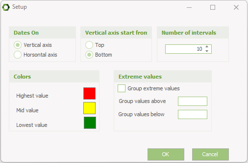
It is possible to tailor the carpet view via the setup menu in the top of the view. When the project is saved these settings are saved along with the project.

The options are:

• Dates on specified axis
• Vertical axis Lowest value from bottom or top
• Number of intervals
• Color of intervals
• Filtering to avoid extreme values

Move time series on

When time series are extended/ copied to another period than actual specified there are two options. The first option is to move the time series on weekly basis (i.e. values in week 2 are moved to week 2 in the following years) and the second is to move on date basis (i.e. values in February 2nd are moved to February 2nd in the following years).

Developing over the years

It is possible to add an index to describe the development of a specified time series. To do this check the “Developing over the years” – option and select a previously created index. For the creation of indexes, see Reference, External Conditions, Indexes. energyPRO develops a time series over time by moving the values as indicated above after moving the values, energyPRO changes the values on a monthly basis according to the selected index.

When the editing windows lower “as graphics”-button is pressed the time series is transformed for the whole planning period. If an index is selected, the index is considered.

Similarly, when the editing windows lower “as carpet”-button is pressed the time series is transformed for the whole planning period and shown as carpet. If an index is selected, the index is taken into account.

“as Graphics” button is pressed a graphic view of the data transformed to the planning period is shown. If an index is selected, the index will be included.

Note that energyPRO tries to keep the time series as simple as possible in order to improve performance, this means that duplicated values is removed. For instance, if coping a time series with 365 daily temperatures you might end up with a time series holding only 320 daily values.

Meteorological time series

Instead of importing climate time series from files and spread sheets, energyPRO offers the opportunity to do this using online data provided by EMD International.

CFSR and CFSR 2 data

CFSR is an abbreviation for Climate Forecast System Reanalysis. CFSR is based on a wide range of data sources, such as surface weather stations, weather balloons, airport reports, commercial aircrafts and satellite measurements.

The CFSR data has a global grid resolution of 0.3 x 0.3 degree and one hour time resolution.

Time series from 1980 to 2010 can be downloaded. Time series from 2011 is available as CFSR 2. CFSR 2 is based on a revised version of the CFSR modelling framework and is run with CFSR 2 has a grid resolution of 0.2 x 0.2 degree and 1 hour time resolution.

The CFSR data has the following data set:

• Air temperature [\(°C\)]
• Solar radiation [\(W/m^2\)]
• Wind speed (10m) [\(m/s\)]
• Precipitation [\(mm\)]
• Humidity [\(\%\)]

ERA5 data

The ERA5 data originates from EU founded project Copernicus Climate Change Service (C3S) and delivered by ECMWF.

Heliosat (SARAH)

The Heliosat (SARAH) data contains surface radiation data. You can select aggregated data or direct and diffuse. Time series from 2016 to now can be downloaded.

If you need other data, typically temperature, you shall combine it with the other data set.

Privacy warning and terms of use acceptance

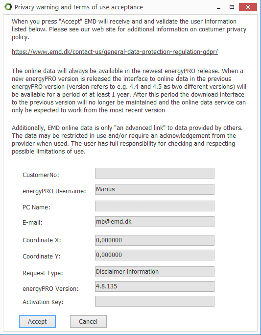
First time downloading online data, you will meet this privacy warning and terms of use acceptance:

This message is also available by clicking the info button in the lower right corner of the window:

Loading time series from online meteorological time series

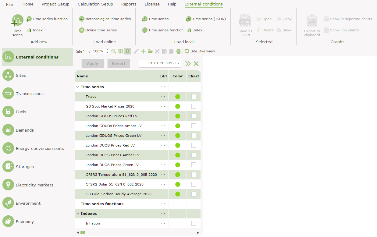
To add time series from online data you can either use the online time series button on the Home toolbar or click on the External conditions button on the left vertical menu, as shown below.

After using either of these methods you will be presented with the window shown below.

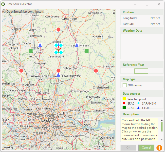
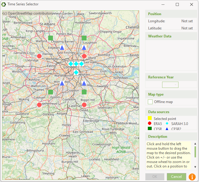
In the window a map is presented on the left-hand side which is used to select the coordinate you wish to add climate time series from. To move the map around you press and hold the left mouse button while dragging the mouse around. You can zoom in by moving the mouse wheel up and zoom out by moving the mouse wheel down.

At the center of the map is shown the four closest points with data for each data type.

Once the nearest data sources are shown you select one of them by clicking on it with the left mouse button.

The next step is to select which climate data you are interested in which is done by clicking the checkboxes in the Weather Data section on the right. For each checked weather source, a time series will be created.

Before the time series can be fetched from the online server and created in energyPRO you need to select a reference year for the data. In the drop-down box you simply select the reference year.

After selecting the reference year, you can go ahead and click Ok to create the time series.

Once you click the Ok button energyPRO will contact the online data server provided by EMD International to fetch the selected climate data. For each weather source that was selected it will create a new time series with default names and symbols. You can rename the time series and symbols as you want.

Online time series

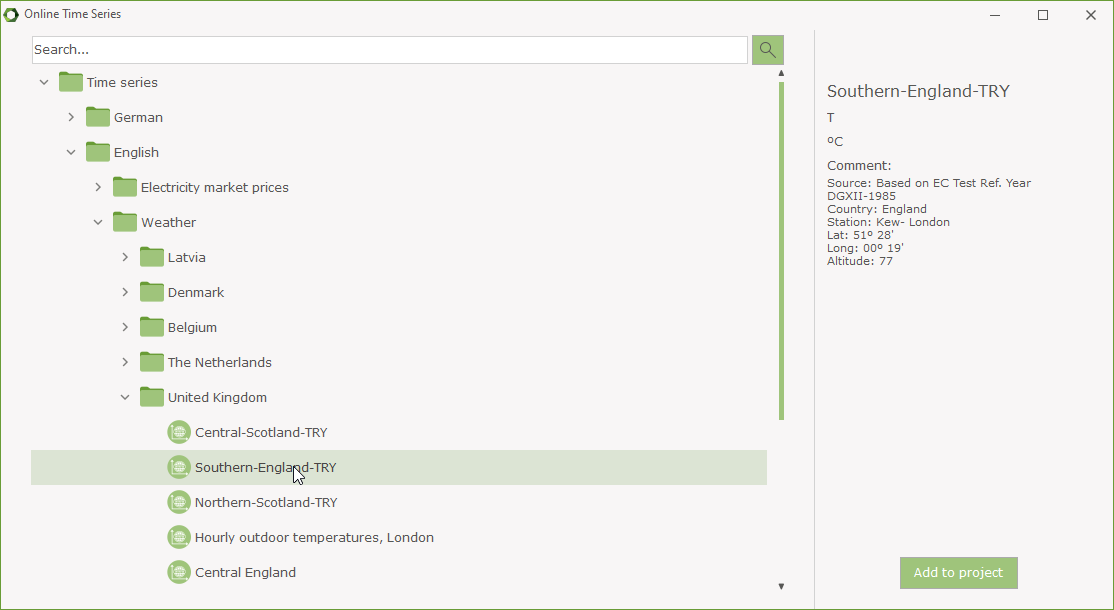
energyPRO offers several hundred time series online. They include a lot of different items, prices, meteorological data, emissions, demand profiles, etc. The are group by country, but you have search options.

Time series functions

Time series functions are primarily meant for modifying existing time series. An example of a time series function is shown below.

Symbol

The symbol is a unique short name of the time series. The symbol is used for referencing the time series elsewhere in the energyPRO. Any time series, time series functions and indexes, used in a project, must use different symbols.

Unit

The unit in which the values in the time series is stated. The unit is for presentation use only.

Where a wind velocity in 10 meters height is modified to wind velocity in 80 meters height.

Function

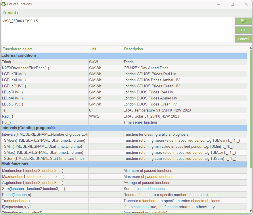
In the function field, you have the option to define a function. If you press the Fx-button in the bottom of the window or double click, you can see which functions are available for defining your time series function and the editing field is enlarged giving the room for viewing all of the function also when having long formulas.

If you need a more detailed description of the functions please see Functions, that serves as a reference-section describing the functions available in formula fields in energyPRO.

In the function shown above a time series is modified. In this example the function modifies a wind speed velocity in 10 meters height to a wind velocity in 80 meters height using a wind gradient exponent of 0.15.

The expression WS(_) refer to a time series, holding hourly values of wind velocity measured in 10 meters height. This time series has the symbol WS. Each value in this time series is modified with the factor (10/80)0.15.

Function to be modified in a conversion table

Below the Function, you have three radio buttons.

An advanced option is to check “Function to be modified in a conversion table”. This gives extra opportunities to modify a time series function.

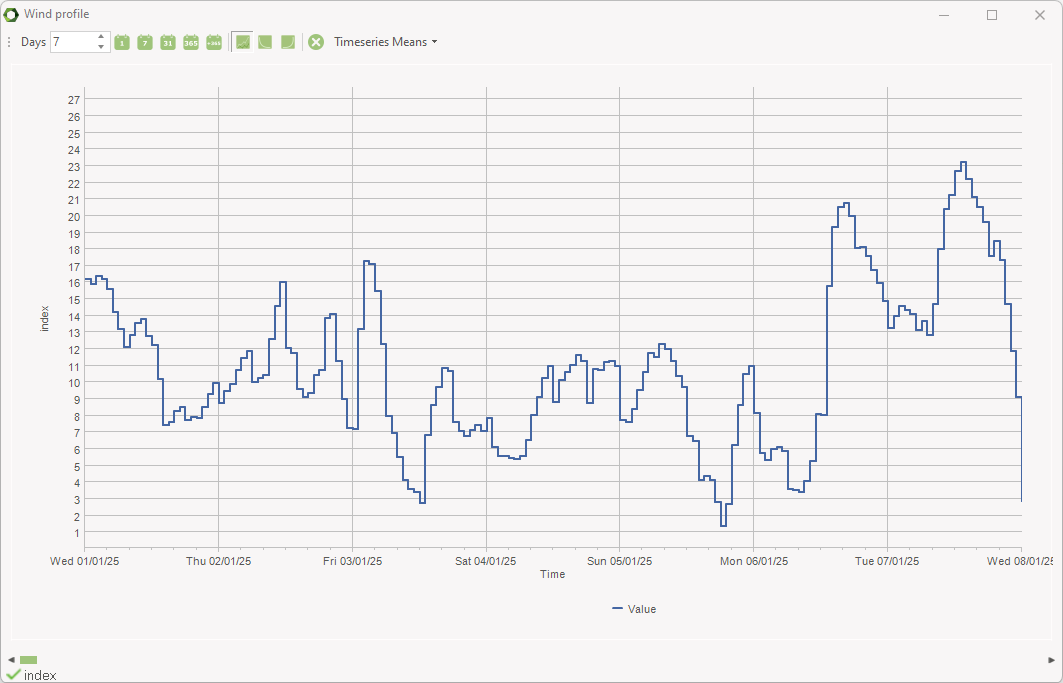
Below is shown a conversion table representing the power curve of a wind turbine. This table modifies the time series function shown above, so the output is a time series function holding variations in energy in wind instead of variations of wind velocity.

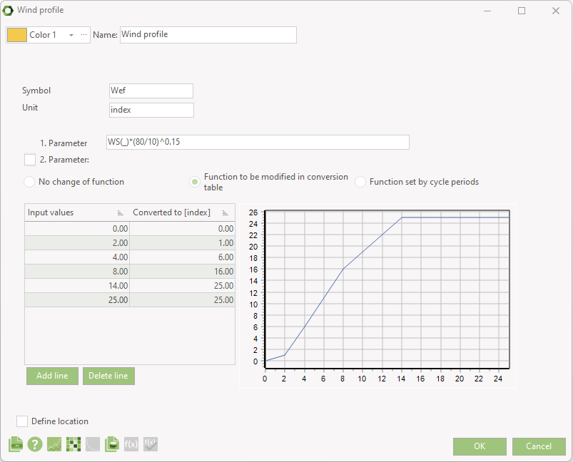
Where a wind velocity in 10 meters height is modified to wind velocity in 80 meters height and finally converted to energy output using a conversion table, which describes the power curve of a wind turbine.

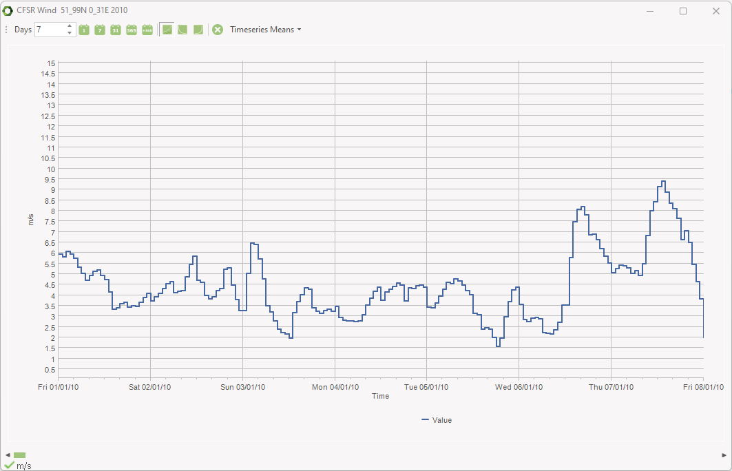
The images below show the graphical representation of the time series function example before and after the conversion table modifies it.

Function to be modified in a 2 dimensional conversion table

Instead of using only one parameter or function, you can enable a second parameter and fill out a 2 dimensional conversion table.

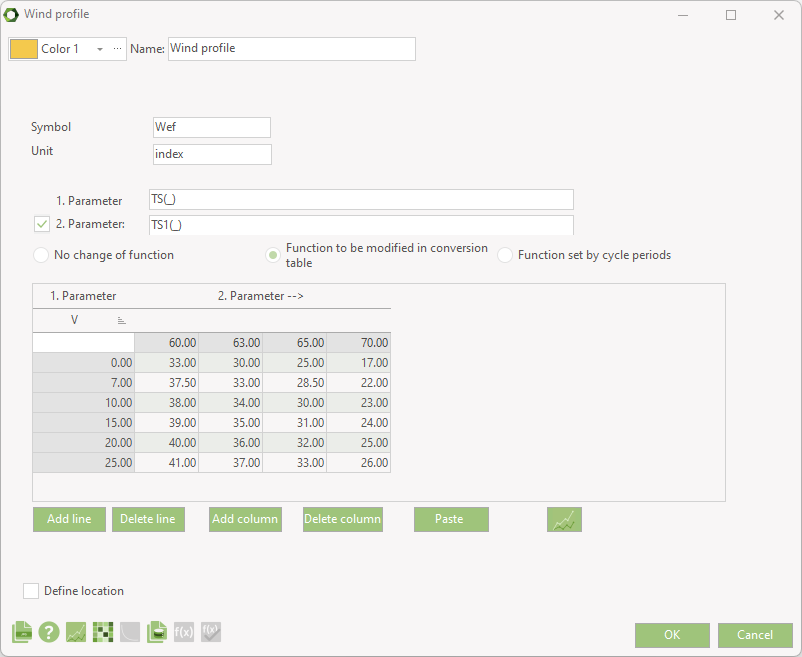
The values of the first parameter is added in the first column, while the values of the second parameter is added in the first row.

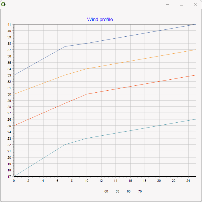
This gives a two dimensional space for the time series function. As graphic it looks like this:

Function set by cycle periods

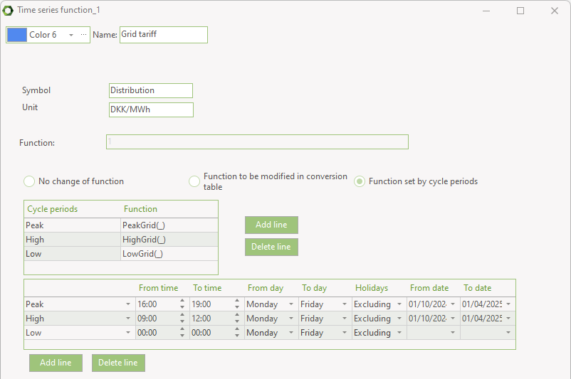
The third option below the function is Function set by cycle periods. This is rather similar to fixed tariff markets, where you can specify fixed market periods.

In the time series function, you define cycle periods and assign a function to each period. Below that you define the periods to be covered by the different cycles.

Indexes

Indexes specify the development of a specific parameter. Indexes are in energyPRO used to describe developments in demands and prices. There are three ways of adding an index to a project.

• Constant annual increase
• Annual increase
• Index

Symbol is a unique short name of the index. The symbol is used for referencing the index elsewhere in the energyPRO. Any time series, time series functions and indexes, used in a project, must have unique symbols.

Constant annual increase. The index changes annually with the percentage typed in. In other words, it changes exponentially and is updated monthly. The index covers the total project period. Index is always 100 on the project start date.

Annual Increase is used if the index has to reflect a shift in rate of change. If the first year in the table is before the project start date then the index on project start date is the value calculated based on input from the table. Index is always 100 on the index start date. The index changes exponentially (yearly update).

Index is used in situations, where you have a series of values (for instance the retail prices index) with values that you want to use if monthly specification is wanted. The index does not change between the indexes typed into the table.

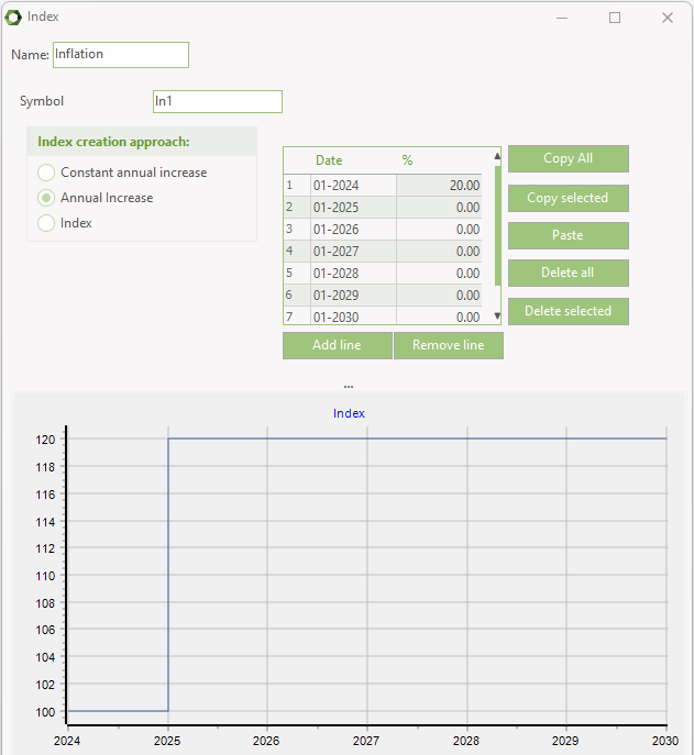
The example shown above is an index used for development of a specific heat demand. Within the first year of the projecting period the heat demand is expected to raise 20% due to connection of new consumers. Annual increase is chosen. In the first projecting year, 2024, the annual increase is 20% and hereafter 0 %. The result is shown in the graphic in the bottom of the window.

Time series overview

When having many time series and time series functions in a project, it can be difficult to grasp them all and it is easy to lose track of how they each depend on one another. For this reason, the overview table with a full list of all the time series and time series functions gives a good overview.

Multiple time series can be added to a graph by using the selection buttons in the "Chart" column.

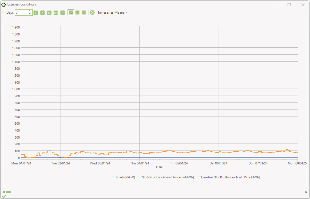
Besides providing a good overview, this table includes several other useful features:

• In the “Function” column, it is possible to change the formula. This is done directly in the table by clicking the formula or from the formula editing window which opens when double clicking the formula or when clicking the F(x)-button.
• The column with check boxes allows the user to select multiple series to be displayed in a graph window – either in separate graphs or in the same graph sharing the same axis as shown in the above figure.
• When selecting a series, its dependents are marked with a green box around the symbol name while its precedents are marked with red.
• In the column with a dropdown menu with a timestamp in the header, you can select a certain time in the planning period and the values of every series, at the selected point in time, will be shown.
• The three columns “Min”, “Max” and “Mean” shows the minimum, maximum and mean values of each series.