Energy conversion units

Energy conversion units – in general

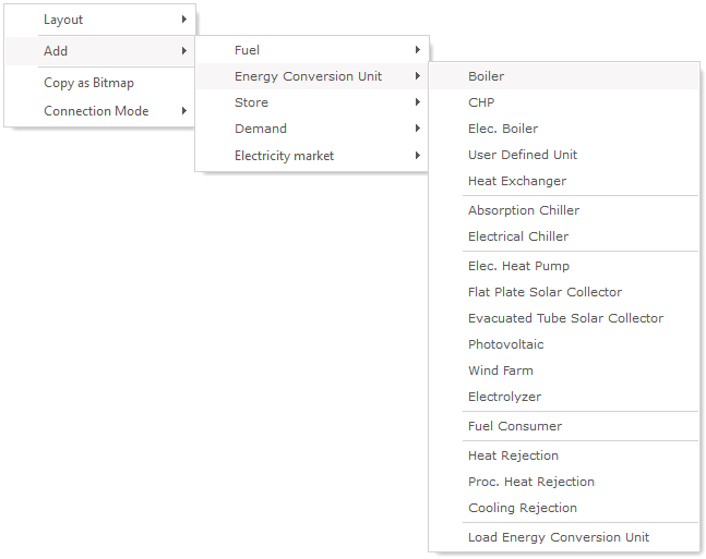
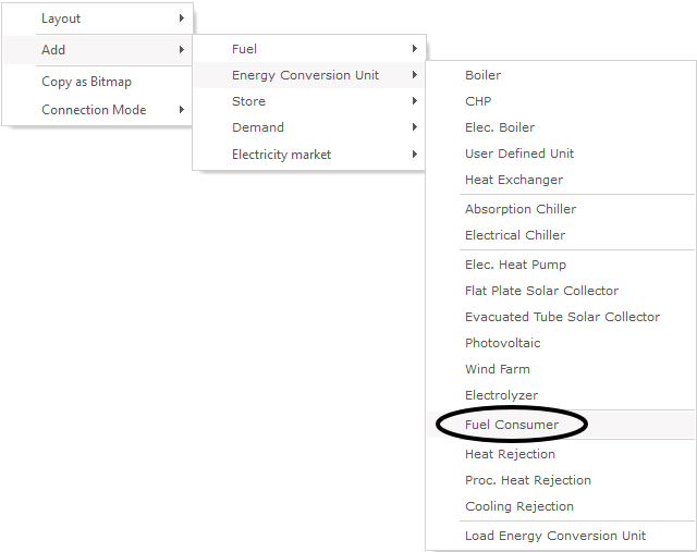
Energy conversion units are added by clicking “Energy conversion unit” on the left-hand vertical menu and selecting an energy conversion unit type from the "Production unit" and "Energy rejection" drop-downs on the tab that appears above. Additionally, this can also be achieved by right-clicking in the Graphical User Mode’s editing window, selecting “Add” and choose “Energy conversion unit”.

There are two types of energy conversion units in energyPRO. Those are

• Production units
• Rejection units

The production units consist of 12 predefined types of units of which one is a user defined type described by load curve(s) and five renewable technologies described with individual editing windows. The Load curve described units are:

• Boiler
• CHP-unit (Combined Heat and Power)
• Electrical boiler
• User defined unit
• Heat Exchanger (From process heat to heat)
• Absorption Chiller
• Electrical Chiller

If the production unit type is consuming (or producing) fuel, one or more fuels defined in a “fuel” sub-folder has to be selected.

The ability to convert energy is described with one or more load curves. Each load curve contains two or more loads, depending on the type of unit. The user-defined unit include all load types. The possible loads are:

• Fuel consumption, any number of fuels
• Heat production
• Heat consumption
• Electric production
• Electric consumption
• Process Heat consumption
• Process Heat production
• Cooling production
• Fuel production, any number of fuels

For advanced users there is a wide scope of options to describe the behaviour of energy units dependent on formulas, the actual production on other production units and time series specified in the “External condition”- folders.

The special treated renewable technologies without load curve description are:

• Electrical heat pump
• Wind farm
• Flat plate solar collector
• Evacuated tube solar collector
• Photovoltaic
• Electrolyser

Production units described by load curves

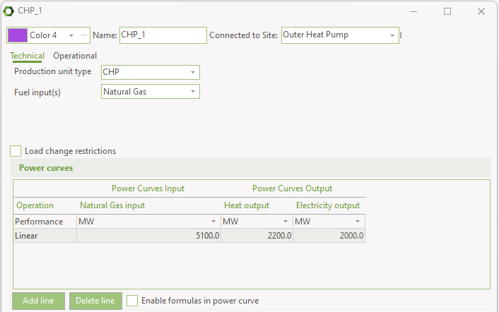
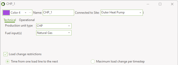
Below is an example of a production unit, in this case a CHP-plant, fuelled with natural gas.

The window has two tabs: Technical and Operational.

Technical

Production unit type

Below the available energy units specified by power curves in energyPRO are shown.

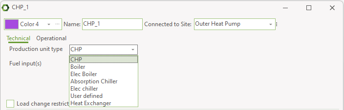
Depending on the production unit type selected, two or more power curves are available. Table 21 shows the power curves available depending on the selected Production unit type.

Production unit	CHP	Boiler	Electrical boiler	Absorption cooling	Electrical cooling	User defined	Heat Exchanger
Fuel consumption	X	X				X
Heat consumption				X		X
Electricity consumption			X		X	X
Process heat consumption						X	X
Heat production	X	X	X			X	X
Process heat production	X	X				X
Electricity production	X					X
Cooling production				X	X	X
Fuel production						X

Note that Process heat production is only available if the “Process Heat” is selected in the “Enable advanced features" section in the “Calculation Setup" tab. Fuel production is only available if “Fuel Production” has been chosen in the same section.

Fuel type

Select one or more fuels in the combo-box. Options are the fuels you have added in your Fuel folder. If “Fuel Production” has been ticked in the “Calculation Setup” and the production unit type is user defined, then a dropdown box called “Fuel output” is added below fuel input dropdown box.

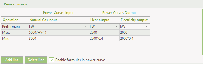
Power curve

In the header of the power curves, the measuring unit is selected. The measuring unit is converted to the default measuring unit of the project before used in the calculation.

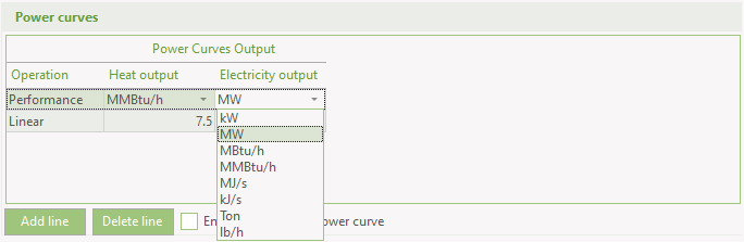
The top line state the maximum loads, while the bottom line states the minimum loads of the energy unit. The loads of the energy unit between the power lines are calculated by linear interpolation. Note that if only one line is stated then a second imaginary line is automatically assumed created with the content of zeroes.

Enable formulas in power curves

This facility gives access to adding formulas in the power curves instead of numbers. The formula will in each time step of the calculation call the formula and return a value.

Note that you can use all the time series created under external conditions and demands you have defined.

For instance, you can make the power curve depend on the ambient temperature. If the symbol for ambient temperature is T, it is referenced by T(_), where the underscore means the value belonging to the time step calculated.

You have the option to define load curves, including

• External conditions. For instance temperature time series
• Demands
• Production on other production units
• Mathematical standard operators

In Functions, there can be found a detailed description of the functions to be used in energyPRO.

Note: The use of formulas in your power curves will normally increase the calculation time considerably.

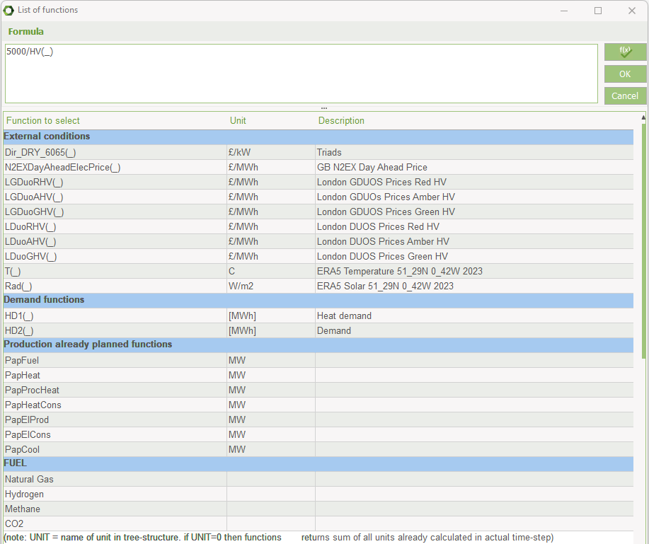
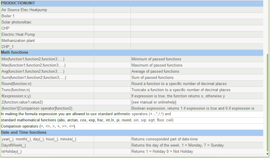
List of Function-buttons

When you push this button a text window will appear. At top, you have an extended editing window, containing the formula. Below the editing window, you can see the available functions and eventually copy and paste them to the power curve. There are six groups of functions. External conditions, demand functions, production already planned functions, fuel, production units, different math functions and date and time functions. The first two references respectively to time series created under external conditions and to the demands. The next two concern the production already planned functions together with the names of the production units to include. The last groups contain basic mathematical functions and date and time functions.

Load change restrictions

When having selected MILP as solver in Project Strategy, Calculation method, you have on the energy conversion unit an option of enabling Load change restrictions.

When enabled you can select between setting the time to go from one load line to the next or setting the maximum load change per timestep.

Selecting Time from one load line to the next gives two load change restriction columns in the power curves:

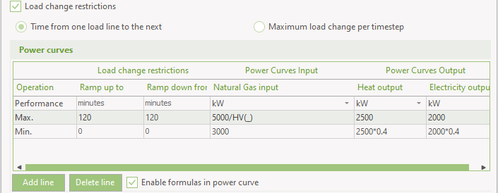
The ramping times can be included for every load line above the minimum load. The times should be entered in minutes. They specify the time it takes to ramp from up from the load line below (“Ramp up to”) and the time it takes to ramp down to the load line below (“Ramp down from”).

Selecting Maximum load change per timestep gives you the option to include a restriction on how much a unit can ramp per timestep.

Below the power curves table, you have a Load change restriction box, where you select any of the energy types:

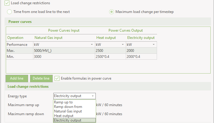
Next, the Maximum ramp up and ramp down load per timestep is specified.

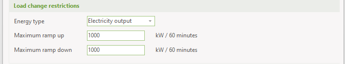
The timestep interval is shown, in this case the calculation step is 1 hour equal to 60 minutes. The measuring unit, in this case kW, is the same as specified in the power curves.

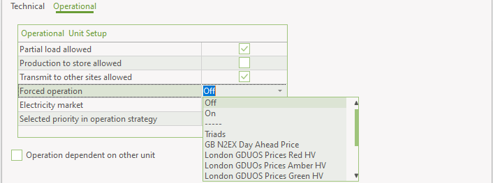
Operational

On the operational tab you have these settings.

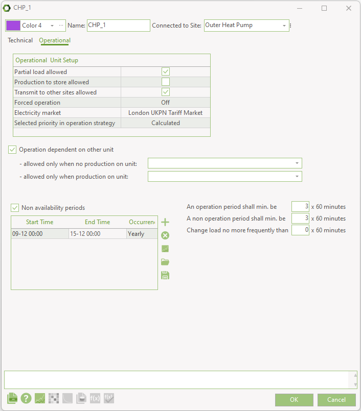
Operational unit setup: Here you have access to the same settings as in the Operation strategy, energy unit setup.

Further, by Forced operation you can select if the energy conversion unit has to operate. The setting can be modified using a dropdown, where you can select between Off (default), On or a time series or time series function.

If the time series has a value higher than zero, the energy conversion unit is forced to operate.

If the energy conversion unit is allowed to part load, the forced operation will apply to the minimum load of the unit.

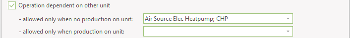
Operation dependent on other unit: With this option checked you can state whether operation on this unit either include or exclude operation on other units. This choice will appear at the bottom of the window as the choices:

• Allowed only when no production on unit
• Allowed only when production on unit.

In both cases, you have the option to specify one of your already created energy units by selecting them in the two combo-boxes

Below is given two examples of how to use this facility.

If you e.g. have an energy unit running on two different fuels, biogas and natural gas, you can define this energy production unit as consisting of two different energy units (biogas engine and natural gas engine). You select the unit you are specifying, e.g. the natural gas engine part is not allowed to run if the biogas engine is already operating.

If you e.g. have an energy unit where you can add an economizer to improve its heat production power output, you can define the economizer as an extra energy unit (modelled as boiler). When selected, the economizer can only be in operation if the belonging energy unit is producing. You then select the unit that have to be operating at the same time as the actual unit that you are editing.

If no energy unit is selected, no restrictions are imposed on the operation.

You have the option of selecting more units. If either one of the selected units are operating, the unit at hand is not allowed to operate (allowed only when no production on unit) or is allowed to operate (allowed only when production on unit)

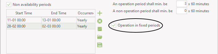
Non-availability periods: By checking the “Non-availability periods”, you get access to a table where you can specify periods, where the actual energy unit is not available for operation. This could for instance be if the unit in a period is out for scheduled maintenance.

It is possible to define the non-availability periods by adding lines stating the occurrences. The possible occurrences are:

• Once
• Yearly
• Monthly
• Weekly
• Daily

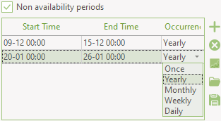
The figure above shows an example where this is the case for 7 days in December and January respectively.

It is possible to construct the non-availability periods by adding lines using a random mix of occurrences (once, daily etc.)

Operation period

You have the option of defining for how long a period at the time the unit minimum shall be in operation and likewise not be in operation.

The periods are specified in timesteps.

If you are using MILP as solver you also have the option of selecting that a load cannot change within a period.

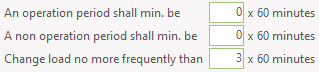
This means that the unit has to be at a certain load for a minimum 3 times the timestep, in this case equal to 3 hours.

The unit is not restricted to being at a specific load line – it can still partially load anywhere between minimum and maximum.

Be aware that if the Change load setting is higher than An operation period.. or A non operation period.. then the Change load no… overrules these settings.

If you in the "Calculation Setup" tab under "Enable advanced features" have enabled "Fixed periods", you have the possibility of forcing energy conversion units to operate in fixed periods:

When enabling Operation in fixed periods, the unit will either have to produce or not produce in all the hours of each fixed period. Each day is split into fixed periods with the length specified in “An operation period shall minimum be”.. This mean that in the example shown above a production period cannot start at e.g. 7 o’clock. It can only start at 00, 03, 06, 09, etc. Likewise the production can only end at the same hours.

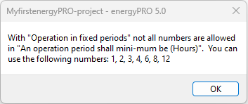
Therefore, the “An operation period shall minimum be” can only have certain values when “Operation in fixed periods” is enabled:

Operation restricted to period: Checking this option gives access to state the period where the unit exist. No specification means that the unit exist in the whole planning period.

Production units not described with load curves

In this section are described production units that are not described with power curves, but internally in energyPRO they are still represented by power curves. Often different in each time step.

Electrical Heat Pump

An electrical heat pump is defined by the electricity consumption and heat output. The ratio between the two is the COP.

The COP (coefficient of performance) of an electrical heat pump is dependant on temperatures and efficiency of the unit.

The electrical heat pump window has two main sections, see below.

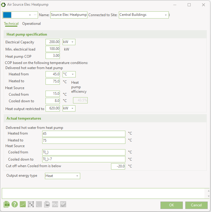
Heat pump specification

Electrical Capacity is the specified electricity load.

Min. electrical load is the minimum electricity load, if part loading is enabled.

Heat pump COP is the COP stated by the supplier under given temperature conditions.

Delivered hot water from heat pump. The temperature of the water coming in (Heated from) and the temperature of the water leaving (Heated to) the heat pump.

Heat Source. The temperatures of the heat source is specified by Cooled from and Cooled down to.

Based on the given temperatures a theoretical Lorentz COP can be calculated.

This theoretical COP is higher than the stated COP. The ratio between the two is the efficiency of the heat pump.

Heat output restricted to is the max achievable heat output capacity. When this value is reached the electrical load will be reduced.

Heat pump efficiency is the calculated efficiency of the heat pump based on the stated COP and the stated temperatures. See “Method of calculating COP and heat capacity in electrical heat pump” for details on how the efficiency is calculated.

Actual temperatures

In this section is specified the actual temperatures of the Delivered hot water from the heat pump and the actual temperatures of the heat source.

These actual temperatures are used to calculate the theoretical COP in the given time step and multiplied by the calculated efficiency a COP is calculated.

This calculated COP is multiplied with the Electrical Capacity resulting in the heat capacity.

With very low temperature differences, the COP can become rather high. With fixed electricity capacity, the heat capacity of the heat pump then becomes high. However, often this is not realizable. When the calculated heat capacity exceeds the Heat output restricted to, the electricity capacity is reduced by dividing the Heat output restricted to with the calculated COP.

If the temperature of the heat source drops below “Cut off when Cooled from is below” the heat pump is not able to operate.

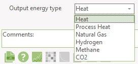
Default of the Output energy type is heat, but if you have enabled process heat and fuel production, you can select the energy type to be either heat, process heat or any of the defined fuels.

Flat plate solar collector and Evacuated tube solar collector

In energyPRO Solar collectors are described by a) Size and position, b) Time series with ambient temperatures and solar radiation and c) Collector and field specific information, see below.

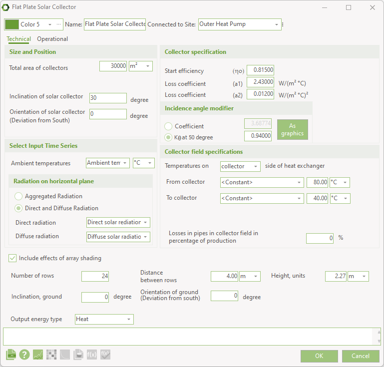
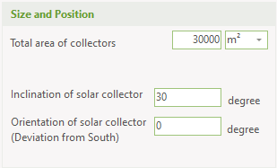
Size and Position

Total area of collectors: Is the aggregated area of the solar collectors.

Inclination of solar collector: This is the tilted angle from ground of the solar collector.

Orientation of solar collector: The orientation of the solar collector is the deviation of the collectors from facing south (northern hemisphere – otherwise deviation from north).

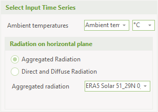
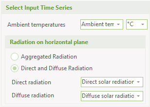
Select Input Time Series

Prerequisites for the calculation of the heat production are time series with ambient temperatures and solar radiation on the horizontal plane.

These time series must be placed in the “External conditions”- folder before modelling the solar collector.

Ambient temperature: Select a time series holding ambient temperatures.

Radiation on horizontal plane: Depending on the available data solar radiation data two options are available. If “Aggregated” solar radiation is available, then select “Aggregated radiation” and select the time series holding these data. If both “Direct” and “Diffuse” is available then select the two time series holding these data, see below.

For the correct calculation of the angle of incidence of beam radiation on the inclined surface and correct correlation between the angle of incidence and the solar radiation, it is important that the location of the time series is specified correct.

This is set in the time series with the solar radiation.

If location is not defined, you will have an error warning. The latitude and longitude are specified in decimal degrees. The latitude has positive values north of equator and negative values south of equator. The longitude has positive values east of Greenwich Mean Time (UTC) and negative values west of Greenwich Mean Time.

Collector and field specification

The solar collectors are specified by several values, defining their technical characteristics. These values are normally found in the data sheets from the manufacturers.

The equation used for the calculations is:

\[ P = A*(I*n_o-a_l*(t_m-t_a)-a_2*(t_m-t_a)^2)*L_p \]

where

\(I\) = Calculated radiation based on the position and radiation time series.

\(t_a\) = Ambient Temperatures found in specified time series.

\(n_o\) = Start efficiency: Start efficiency is also called “Conversion factor”. The collectors start efficiency, where the fluid temperature equals the ambient temperature.

\(a_1\) = Loss coefficient (a1)

\(a_2\) = Loss coefficient (a2)

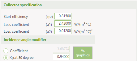
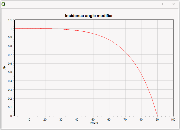
Incidence angle modifier (\(K_\theta\)): Refers to the change in performance as the sun's angle in relation to the collector surface changes. The IAM is used for the calculation of, found in the equation above.

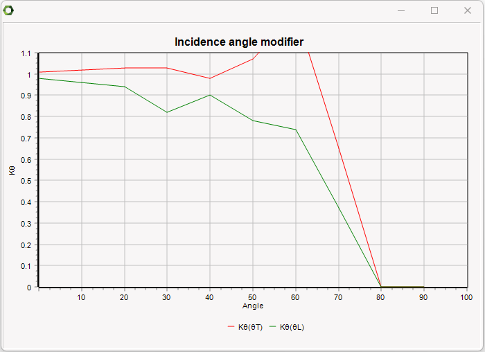
The Evacuated Tube Solar Collector differs from the flat plate solar collector when it comes to the Incidence Angle modifier:

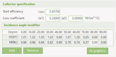
Evacuated tube collectors are optically non-symmetric. The incidence angle modifier is divided into a longitude and transversal IAM. The above values look like this as graphic:

\(t_m\) = Collector temperature: The average temperature of the collectors on the collector side. This temperature is defined by a forward temperature (the temperature of the water leaving the collector), \(t_{from}\) and a return temperature (the temperature of the water entering the collector), \(t_{to}\). These values can either be fixed or referring to an external time series. Most often these temperatures are known on the demand side of the heat exchanger, but in the calculations it is the temperature on the collector side of the heat exchanger that is needed. So if you know the temperature on the demand side you can select that in the user interface and then you also have to specify the temperature drop over the heat exchanger, \(t_{hx}\). The complete equation for calculating \(t_m\) is then:

\[ t_m = (t_{from} + t_{to})/2 + t_{hx} \]

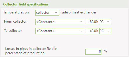
\(L_p\) = Losses in pipes: This represents the loss in the pipes in the collector field. The loss is simply given as a percentage of the heat production.

Array shading

Often, large scale solar collector or photo voltaic systems will be mounted on the ground in rows which results in array shading. In other words, solar collectors in one row will produce shade on the row behind it (compared to the sun). In energyPRO the effect of array shading is included by specifying the following parameters:

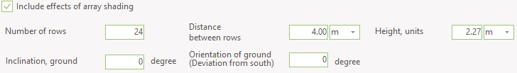
• Number of rows: The number of rows in the array
• Distance between rows: The distance between each row
• Height, units: The height of each solar collector
• Inclination, ground: The inclination of the ground in degrees. 0 means a flat surface.
• Orientation of ground: The orientation of the ground relative to directly south.

These parameters are used to calculate the effect of array shading on direct (beam), diffuse and reflected radiation.

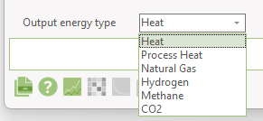
Output energy type

Default the Output energy type is heat, but if you have enabled process heat and fuel production, you can select the energy type to be either heat, process heat or any of the defined fuels.

Photovoltaic

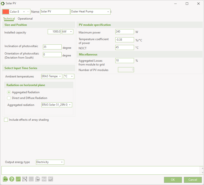
In energyPRO solar Photovoltaic is described by a) Size and position, b) Time series with ambient temperatures and solar radiation and c) a PV module specific information, and d) Miscellaneous, see below.

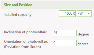
Size and Position

Total Installed capacity: Is the aggregated capacity of installed PV panels.

Latitude UTM: Is the Latitude of the Photovoltaic in UTM coordinates.

Inclination of photovoltaic: This is the tilted angle from ground of the PV panels.

Orientation of photovoltaic: The orientation of the photovoltaic is the deviation of the PV panels from facing south (northern hemisphere – otherwise deviation from north).

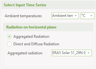
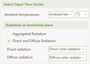
Select Input Time Series

Prerequisites for the calculation of the heat production are time series with ambient temperatures and solar radiation on the horizontal plane.

These time series must be placed in the “External conditions”- folder before modelling the photovoltaic.

Ambient temperature: Select a time series holding ambient temperatures.

Radiation on horizontal plane: Depending on the available solar radiation data two options are available. If “Aggregated” solar radiation is available, then select “Aggregated radiation” and select the time series holding these data. If both “Direct” and “Diffuse” is available then select the two time series holding these data, see below.

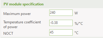
PV module specification

The PV module is described by three parameters, normally found on the manufacturers’ data sheets.

Maximum power: The “Maximum power” from the PV panel under standard conditions. This value is not used in the energy conversion but only to calculate the number of panels.

Temperature coefficient of power: This coefficient specifies how the power productions from the panels react to changes operating temperature.

NOCT: Normal Operating Cell Temperature

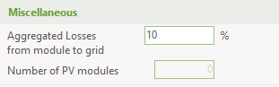
Miscellaneous

Aggregated losses from module to grid: This value represents the losses from module to grid and encompasses PV array losses, cable losses, inverter losses etc.

Like most other input fields in the PV module, you can define the aggregated losses from module to grid as a formula. Special for this field is that when entering the list of functions, you have access to a function called PVdc. With this you can include a formula taking the efficiency of the inverter into account.

Number of values: The calculated number of panels based on installed capacity and the Maximum power from the PV module specification.

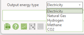
Default the Output energy type is electricity, but if you have enabled fuel production, you can select the energy type to be either electricity or any of the defined fuels.

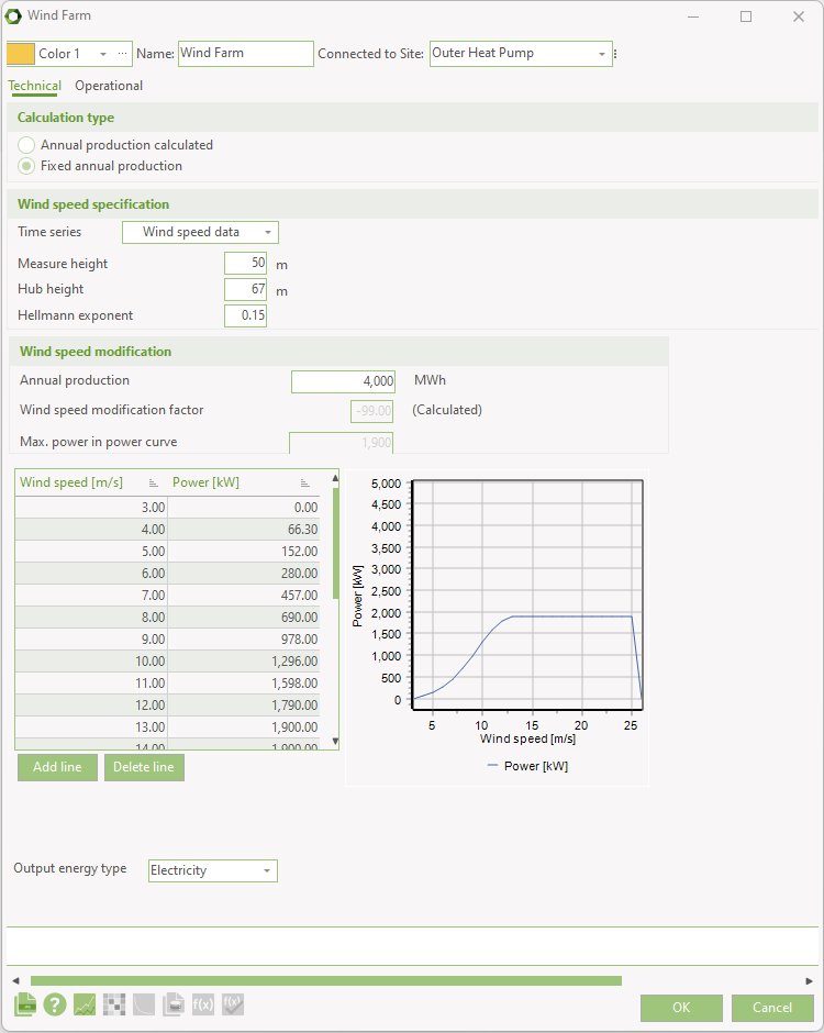
Wind farm

The wind farm is a specialised energy unit having the general energy unit properties such as “non availability periods”, the “operation dependent on other unit”-option and the “restricted to period”-option.

The wind farm uses an external time series with measured wind speed and a wind farm power curve to calculate electric production from the wind farm. The time series with wind speed must be present in the “External conditions”-folder, and the power curve must be specified in the wind farm editing window.

Calculation type

There are two approaches for calculation of wind farms in energyPRO.

1. Annual production calculated, divided into two sub cases
   1. Park power curve is used directly
   2. Power curve is scaled to another level
2. Fixed annual production (wind speed is scaled)

All approaches require that a time series holding wind speed is available and present in the “External conditions”-folder.

Annual production calculated. In this case the productions from the wind farm are calculated based on the wind speed specification and power curve of the wind farm. As an advanced setting, there are options to scale the power curve and thereby the production.

Fixed annual production. This option serves to distribute a desired annual production given a specified wind farm power curve. All wind speeds specified through “Wind speed specification” (see below) are scaled by the modification factor that makes agreement between the annual production, the power curve and the wind speeds. This factor is found through iterations.

Wind speed specification

The wind speed at hub height is defined through the following parameters, which is used for converting the wind speed in measure height to wind speed at hub height.

1. A time series holding the wind speed
2. The measure height of the time series
3. The hub height of the turbines
4. The Hellmann exponent

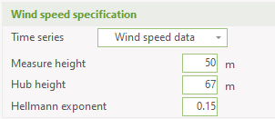
The time series must be established in “External conditions” prior to the specification.

Specification of power curve

The power curve consists of a data set of values containing the wind speed and the corresponding power output from the turbines. In the calculation, the power output is assumed to be linear between two data elements. The power curve is specified through a data table and shown on a corresponding graph, see below.

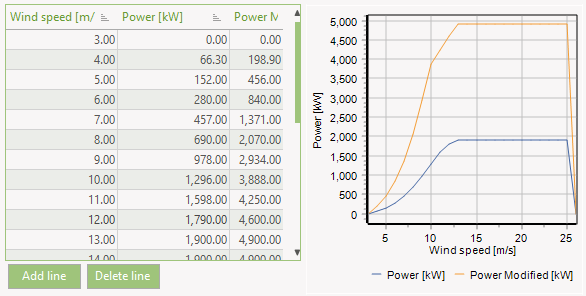
The functionalities of the table are comparable to the other energyPRO tables. This includes unlimited number of values, add line and delete line buttons. Data is added by typing data into the table or it can be pasted via the clipboard. It is possible to copy a calculated wind park curve from WindPro via clipboard to the wind farm power curve in energyPRO, see below.

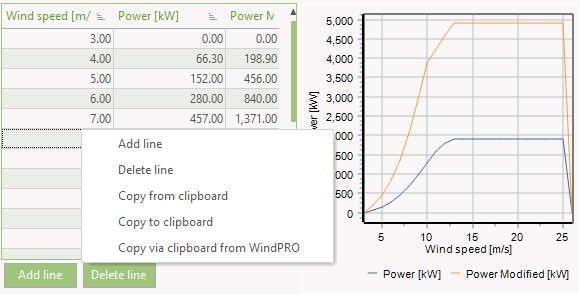
Values can be copied from clipboard, including park power curve calculated in WindPro.

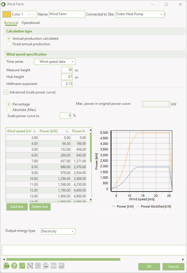
The content of the wind farm editing-window if “Annual production calculated” is selected, is shown below.

This window contains the data described in this window, plus an advanced option.

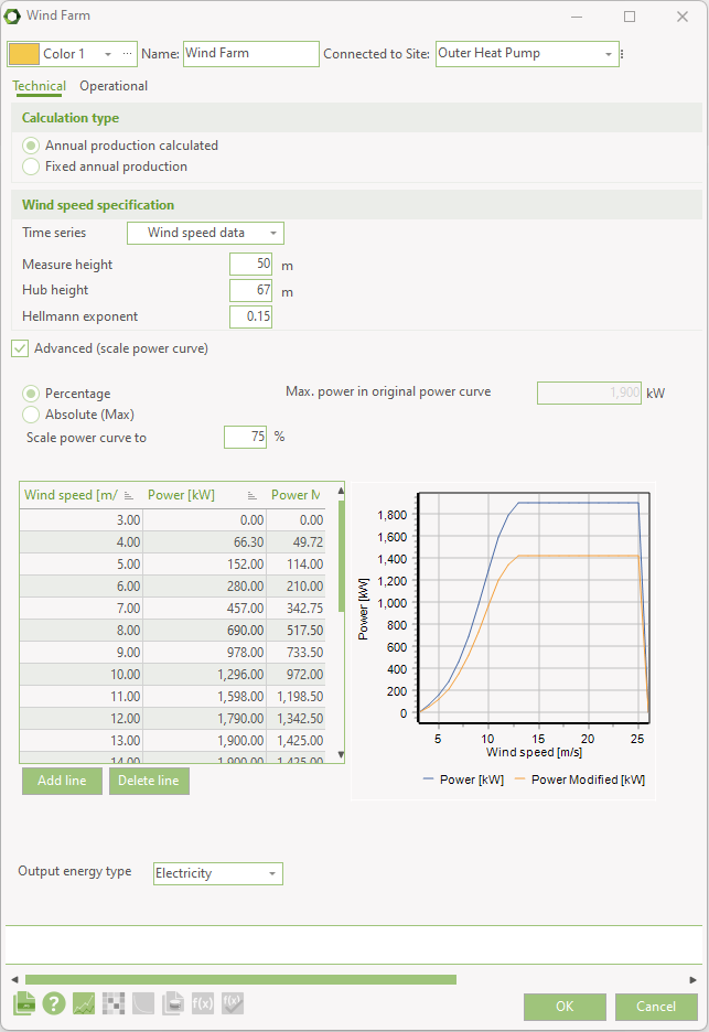
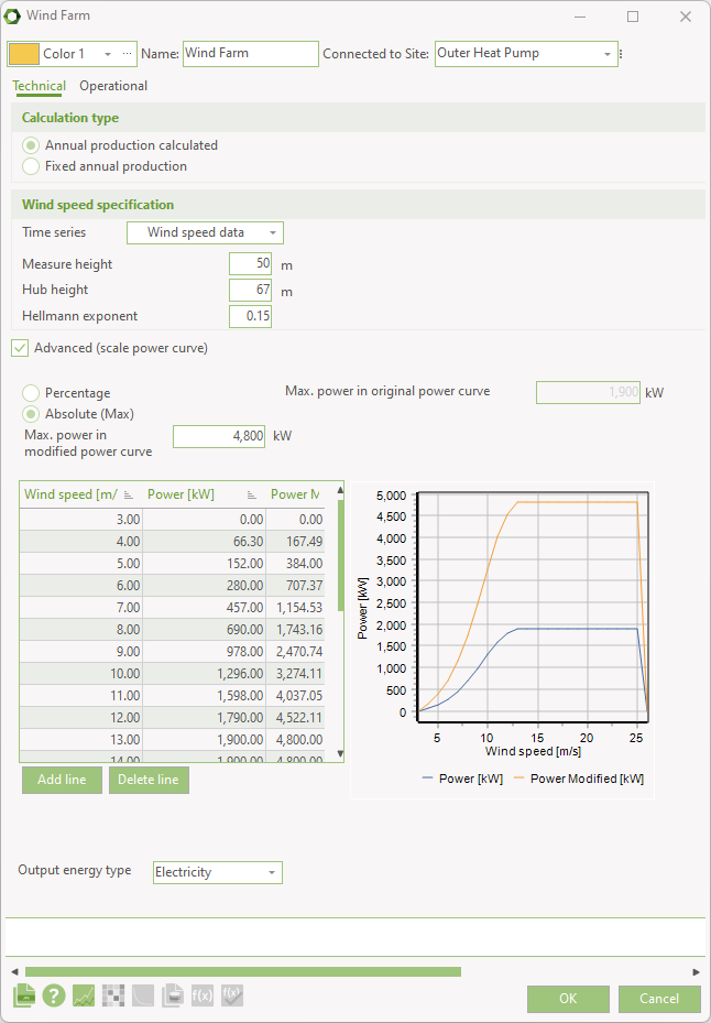
Annual production calculated (power curve scaled)

An example of this is shown below. Notice that the power curve now has a new resulting power curve both in the table presentation and in the graphic representation. There are two variants. It is possible to scale using a percentage or a new max power curve value, see both images below.

Fixed Annual production

If Fixed annual production is selected then the Annual production and the wind farm power curve is specified (e.g. calculated in WindPro). Given the power curve and a stated annual production all wind speed values are scaled by a factor. This factor is calculated, and is used when calculating the production at any time. See the description in Methods, Wind Farms.

Electrolyser

The electrolysis unit allows you to model the production of hydrogen through the usage of electricity and water in energyPRO. Besides electricity consumption and hydrogen production you can model the water consumption and oxygen production of two different electrolysis technologies: alkaline electrolysis (AE) and polymer membrane electrolysis (PEM).

Allow fuel producing units

First step is to allow fuel production. Go to the Calculation Setup tab and in Enable advanced features Choose “Fuel production”.

Electrolyser window

The electrolyser looks as follows.

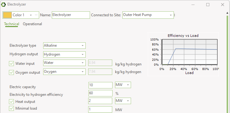
To determine the energetic efficiency and thereby the relation between energy consumption and production, the type of electrolyser is established. In the Electrolyser drop-down menu either “Alkaline” or “Polymer Electrolyte Membrane” can be chosen. Furthermore, the electric capacity and the Electricity to Hydrogen efficiency need to be entered.

It is mandatory to have selected a fuel for Hydrogen output. It is optional to include water input and oxygen output.

The Hydrogen, water and oxygen fuels need to be defined in kg and the heat value of the hydrogen fuel has to be 33.3 kWh/kg. It is recommended to load the predefined fuels from the energyPRO data fuel folder.

Additionally, a heat production and a minimal load can be added by checking the respective checkboxes. The heat production is entered as an absolute value, while the minimal load as entered as a percentage of electric capacity. The minimal load is referring to the lowest part load that the electrolyser can run at.

The entered minimal load is not allowed to be higher than 25% for Alkaline and 27% for Polymer Membrane Electrolysis of the electric capacity, to be entered as electric capacity in MW.

The entered heat output, as heat production capacity during nominal load, should not exceed:

\[ (1 - \eta{\_}(H_2,{out},{peak})\cdot {E\_cap} \]

Where:

\(\eta{\_}(H_2,{out},{peak})\) is the highest possible efficiency of electric input to hydrogen production and not the nominal efficiency.

\({E\_cap}\) is the nominal electric capacity of the electrolyser.

Rejection units

A rejection unit is e.g. used in situations, where electricity demands require electricity production from co-generating engines, while the heat produced by the cooling of the engines cannot be utilized.

If a heat rejection unit is inserted, you must remember to select, which of the production units that have access to the heat rejection unit. This selection is done in the “Operation Strategy” editing window.

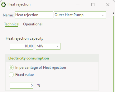
Heat rejection capacity: Here you state the heat rejection capacity.

Electricity consumption: An eventual electricity consumption can be stated either as a fixed percentage of the actual heat rejection or as a constant consumption when the unit is operated independent of the load.

Note that the heat rejection is post processed the energy conversion calculation. The consequence hereof is that there will be a residual import of electricity when demand and productions has been balanced.

Operation restricted to period: By checking this option you got access to state the period where the unit exist. No specification means that the unit exist in the whole planning period.

Non-availability periods: By checking the “Non availability periods”, you get access to a table where you can specify periods, where the actual energy unit is not available for operation.

The cooling and process heat rejection units are similar to the heat rejection unit.

Fuel demand

Similar to heat, process heat, cooling and electricity you can specify fuel demand. Technically, the fuel demand is treated similar to an energy conversion unit. This means that when adding a fuel demand, you have to go by the add energy conversion unit menu, where you select fuel consumer.

In the fuel consumption window, you select the fuel, select measuring unit and set a function for the demand.

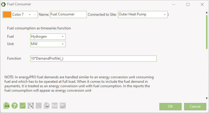
As written in the window, the fuel demand is handled similar to an energy conversion unit and appears as such in the reports and payments.